
A Data frame is a two-dimensional data structure, i.e., data is aligned in a tabular fashion in rows and columns.
Features of DataFrame
- Potentially columns are of different types
- Size – Mutable
- Labeled axes (rows and columns)
- Can Perform Arithmetic operations on rows and columns
Structure
Let us assume that we are creating a data frame with student’s data.
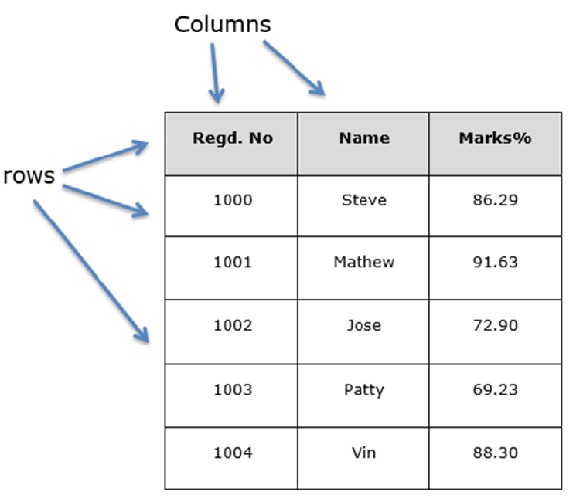
You can think of it as an SQL table or a spreadsheet data representation.
pandas.DataFrame
A pandas DataFrame can be created using the following constructor −
pandas.DataFrame( data, index, columns, dtype, copy)
The parameters of the constructor are as follows −
| S.No | Parameter & Description |
|---|---|
| 1 | data
data takes various forms like ndarray, series, map, lists, dict, constants and also another DataFrame. |
| 2 | index
For the row labels, the Index to be used for the resulting frame is Optional Default np.arrange(n) if no index is passed. |
| 3 | columns
For column labels, the optional default syntax is - np.arrange(n). This is only true if no index is passed. |
| 4 | dtype
Data type of each column. |
| 4 | copy
This command (or whatever it is) is used for copying of data, if the default is False. |
Create DataFrame
A pandas DataFrame can be created using various inputs like −
- Lists
- dict
- Series
- Numpy ndarrays
- Another DataFrame
In the subsequent sections of this chapter, we will see how to create a DataFrame using these inputs.
Create an Empty DataFrame
A basic DataFrame, which can be created is an Empty Dataframe.
Example
#import the pandas library and aliasing as pd
import pandas as pd
df = pd.DataFrame()
print df
Its output is as follows −
Empty DataFrame
Columns: []
Index: []
Create a DataFrame from Lists
The DataFrame can be created using a single list or a list of lists.
Example 1
import pandas as pd
data = [1,2,3,4,5]
df = pd.DataFrame(data)
print df
Its output is as follows −
     0
0    1
1    2
2    3
3    4
4    5
Example 2
import pandas as pd
data = [['Alex',10],['Bob',12],['Clarke',13]]
df = pd.DataFrame(data,columns=['Name','Age'])
print df
Its output is as follows −
      Name      Age
0     Alex      10
1     Bob       12
2     Clarke    13
Example 3
import pandas as pd
data = [['Alex',10],['Bob',12],['Clarke',13]]
df = pd.DataFrame(data,columns=['Name','Age'],dtype=float)
print df
Its output is as follows −
      Name     Age
0     Alex     10.0
1     Bob      12.0
2     Clarke   13.0
Note − Observe, the dtype parameter changes the type of Age column to floating point.
Create a DataFrame from Dict of ndarrays / Lists
All the ndarrays must be of same length. If index is passed, then the length of the index should equal to the length of the arrays.
If no index is passed, then by default, index will be range(n), where n is the array length.
Example 1
import pandas as pd
data = {'Name':['Tom', 'Jack', 'Steve', 'Ricky'],'Age':[28,34,29,42]}
df = pd.DataFrame(data)
print df
Its output is as follows −
      Age      Name
0     28        Tom
1     34       Jack
2     29      Steve
3     42      Ricky
Note − Observe the values 0,1,2,3. They are the default index assigned to each using the function range(n).
Example 2
Let us now create an indexed DataFrame using arrays.
import pandas as pd
data = {'Name':['Tom', 'Jack', 'Steve', 'Ricky'],'Age':[28,34,29,42]}
df = pd.DataFrame(data, index=['rank1','rank2','rank3','rank4'])
print df
Its output is as follows −
         Age    Name
rank1    28      Tom
rank2    34     Jack
rank3    29    Steve
rank4    42    Ricky
Note − Observe, the index parameter assigns an index to each row.
Create a DataFrame from List of Dicts
List of Dictionaries can be passed as input data to create a DataFrame. The dictionary keys are by default taken as column names.
Example 1
The following example shows how to create a DataFrame by passing a list of dictionaries.
import pandas as pd
data = [{'a': 1, 'b': 2},{'a': 5, 'b': 10, 'c': 20}]
df = pd.DataFrame(data)
print df
Its output is as follows −
    a    b      c
0   1   2     NaN
1   5   10   20.0
Note − Observe, NaN (Not a Number) is appended in missing areas.
Example 2
The following example shows how to create a DataFrame by passing a list of dictionaries and the row indices.
import pandas as pd
data = [{'a': 1, 'b': 2},{'a': 5, 'b': 10, 'c': 20}]
df = pd.DataFrame(data, index=['first', 'second'])
print df
Its output is as follows −
        a   b       c
first   1   2     NaN
second  5   10   20.0
Example 3
The following example shows how to create a DataFrame with a list of dictionaries, row indices, and column indices.
import pandas as pd
data = [{'a': 1, 'b': 2},{'a': 5, 'b': 10, 'c': 20}]

#With two column indices, values same as dictionary keys
df1 = pd.DataFrame(data, index=['first', 'second'], columns=['a', 'b'])

#With two column indices with one index with other name
df2 = pd.DataFrame(data, index=['first', 'second'], columns=['a', 'b1'])
print df1
print df2
Its output is as follows −
#df1 output
         a  b
first    1  2
second   5  10

#df2 output
         a  b1
first    1  NaN
second   5  NaN
Note − Observe, df2 DataFrame is created with a column index other than the dictionary key; thus, appended the NaN’s in place. Whereas, df1 is created with column indices same as dictionary keys, so NaN’s appended.
Create a DataFrame from Dict of Series
Dictionary of Series can be passed to form a DataFrame. The resultant index is the union of all the series indexes passed.
Example
import pandas as pd

d = {'one' : pd.Series([1, 2, 3], index=['a', 'b', 'c']),
      'two' : pd.Series([1, 2, 3, 4], index=['a', 'b', 'c', 'd'])}

df = pd.DataFrame(d)
print df
Its output is as follows −
      one    two
a     1.0    1
b     2.0    2
c     3.0    3
d     NaN    4
Note − Observe, for the series one, there is no label ‘d’ passed, but in the result, for the d label, NaN is appended with NaN.
Let us now understand column selection, addition, and deletion through examples.
Column Selection
We will understand this by selecting a column from the DataFrame.
Example
import pandas as pd

d = {'one' : pd.Series([1, 2, 3], index=['a', 'b', 'c']),
      'two' : pd.Series([1, 2, 3, 4], index=['a', 'b', 'c', 'd'])}

df = pd.DataFrame(d)
print df ['one']
Its output is as follows −
a     1.0
b     2.0
c     3.0
d     NaN
Name: one, dtype: float64
Column Addition
We will understand this by adding a new column to an existing data frame.
Example
import pandas as pd

d = {'one' : pd.Series([1, 2, 3], index=['a', 'b', 'c']),
      'two' : pd.Series([1, 2, 3, 4], index=['a', 'b', 'c', 'd'])}

df = pd.DataFrame(d)

# Adding a new column to an existing DataFrame object with column label by passing new series

print ("Adding a new column by passing as Series:")
df['three']=pd.Series([10,20,30],index=['a','b','c'])
print df

print ("Adding a new column using the existing columns in DataFrame:")
df['four']=df['one']+df['three']

print df
Its output is as follows −
Adding a new column by passing as Series:
     one   two   three
a    1.0    1    10.0
b    2.0    2    20.0
c    3.0    3    30.0
d    NaN    4    NaN

Adding a new column using the existing columns in DataFrame:
      one   two   three    four
a     1.0    1    10.0     11.0
b     2.0    2    20.0     22.0
c     3.0    3    30.0     33.0
d     NaN    4     NaN     NaN
Column Deletion
Columns can be deleted or popped; let us take an example to understand how.
Example
# Using the previous DataFrame, we will delete a column
# using del function
import pandas as pd

d = {'one' : pd.Series([1, 2, 3], index=['a', 'b', 'c']),
     'two' : pd.Series([1, 2, 3, 4], index=['a', 'b', 'c', 'd']),
     'three' : pd.Series([10,20,30], index=['a','b','c'])}

df = pd.DataFrame(d)
print ("Our dataframe is:")
print df

# using del function
print ("Deleting the first column using DEL function:")
del df['one']
print df

# using pop function
print ("Deleting another column using POP function:")
df.pop('two')
print df
Its output is as follows −
Our dataframe is:
      one   three  two
a     1.0    10.0   1
b     2.0    20.0   2
c     3.0    30.0   3
d     NaN     NaN   4

Deleting the first column using DEL function:
      three    two
a     10.0     1
b     20.0     2
c     30.0     3
d     NaN      4

Deleting another column using POP function:
   three
a  10.0
b  20.0
c  30.0
d  NaN
Row Selection, Addition, and Deletion
We will now understand row selection, addition and deletion through examples. Let us begin with the concept of selection.
Selection by Label
Rows can be selected by passing row label to a loc function.
import pandas as pd

d = {'one' : pd.Series([1, 2, 3], index=['a', 'b', 'c']),
     'two' : pd.Series([1, 2, 3, 4], index=['a', 'b', 'c', 'd'])}

df = pd.DataFrame(d)
print df.loc['b']
Its output is as follows −
one 2.0
two 2.0
Name: b, dtype: float64
The result is a series with labels as column names of the DataFrame. And, the Name of the series is the label with which it is retrieved.
Selection by integer location
Rows can be selected by passing integer location to an iloc function.
import pandas as pd

d = {'one' : pd.Series([1, 2, 3], index=['a', 'b', 'c']),
     'two' : pd.Series([1, 2, 3, 4], index=['a', 'b', 'c', 'd'])}

df = pd.DataFrame(d)
print df.iloc[2]
Its output is as follows −
one   3.0
two   3.0
Name: c, dtype: float64
Slice Rows
Multiple rows can be selected using ‘ : ’ operator.
import pandas as pd

d = {'one' : pd.Series([1, 2, 3], index=['a', 'b', 'c']),
    'two' : pd.Series([1, 2, 3, 4], index=['a', 'b', 'c', 'd'])}

df = pd.DataFrame(d)
print df[2:4]
Its output is as follows −
      one    two
c     3.0     3
d     NaN     4
Addition of Rows
Add new rows to a DataFrame using the append function. This function will append the rows at the end.
import pandas as pd

df = pd.DataFrame([[1, 2], [3, 4]], columns = ['a','b'])
df2 = pd.DataFrame([[5, 6], [7, 8]], columns = ['a','b'])

df = df.append(df2)
print df
Its output is as follows −
   a  b
0  1  2
1  3  4
0  5  6
1  7  8
Deletion of Rows
Use index label to delete or drop rows from a DataFrame. If label is duplicated, then multiple rows will be dropped.
If you observe, in the above example, the labels are duplicate. Let us drop a label and will see how many rows will get dropped.
import pandas as pd

df = pd.DataFrame([[1, 2], [3, 4]], columns = ['a','b'])
df2 = pd.DataFrame([[5, 6], [7, 8]], columns = ['a','b'])

df = df.append(df2)

# Drop rows with label 0
df = df.drop(0)

print df
Its output is as follows −
  a b
1 3 4
1 7 8


###############################DATA FRAMES #####################
import pandas as pd
import numpy as np
df=pd.DataFrame()
print(df)
# List
l=[1,2,3,4]
df=pd.DataFrame(l,columns=['age'],index=["one","two","three","four"])
print(df)
# List of lists
df=pd.DataFrame([['a',21],['b',20],['c',22]],columns=["name",'age'],index=["one","two","three"])
print(df)
# Dictionary
df=pd.DataFrame({'name':['a','b','c'],'age':[21,20,22]},index=["one","two","three"])
print(df)
# List of dictionaries
df=pd.DataFrame([{'a':21,'b':20,'c':22},{'a':19,'b':18,'c':17}],index=["one","two"])
print(df)
# Select Column
print(df['a'])
# Column Addition
print(df['a']+df['b'])
#Append new column
df['d']=df['a']+df['b']
print(df)
# Delete column
del df['d']
print(df)
# Select row
print(df.loc['one'])
# row Addition
#print(df['one']+df['two'])
# Delete column
df=df.drop('one')
print(df)
################assignment#############################
import pandas as pd
import numpy as np
labels= ['name','roll_no','s1','s2','s3','s4']
#df=pd.DataFrame([{"x1",123,50,60,65,70],["x2",124,53,24,65,80],["x3",125,57,70,45,90]]}
#print(df)
df=pd.DataFrame([{'name':'x1','roll_no':123,'s1':50,'s2':50,'s3':50},
{'name':'x2','roll_no':124,'s1':55,'s2':57,'s3':56},])
#df=pd.DataFrame[d,columns=('name','roll_no','s1','s2','s3','s4')]
#df.columns = [labels]
print(df)
print(df['s1'])
print(df['s2'])
print(df['s1']+df["s2"])
df['total']=df['s1']+df['s2']+df['s3']
print(df)
df['avg']=df['total']/3
print(df)
bins=[0,50,60,70,80,90,100]
grade=['F','E','D','C','B','A']
df['Grade']=pd.cut(df['avg'],bins, labels=grade)
#df['grade']=df['avg']
print(df)
#########################
Python | Pandas DataFrame
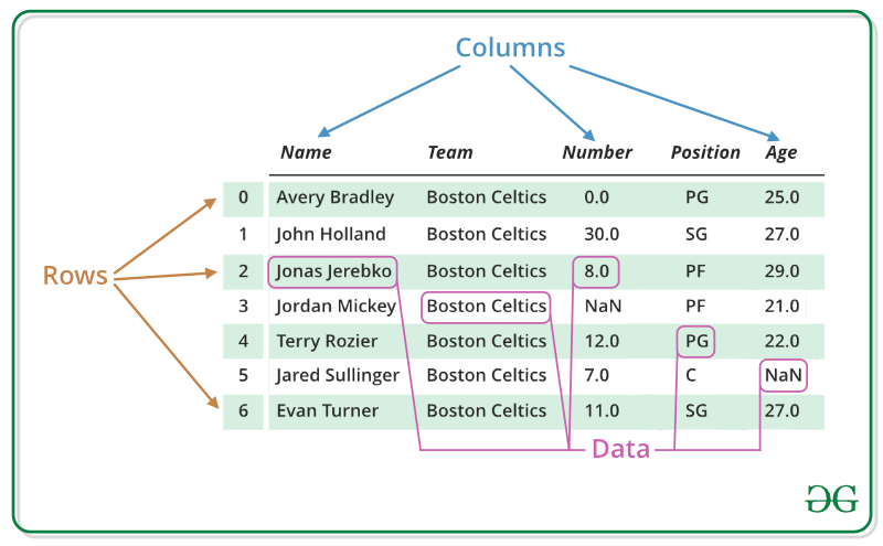
Pandas DataFrame is two-dimensional size-mutable, potentially heterogeneous tabular data structure with labeled axes (rows and columns). A Data frame is a two-dimensional data structure, i.e., data is aligned in a tabular fashion in rows and columns. Pandas DataFrame consists of three principal components, the data, rows, and columns.
We will get a brief insight on all these basic operation which can be performed on Pandas DataFrame :
- Creating a DataFrame
- Dealing with Rows and Columns
- Indexing and Selecting Data
- Working with Missing Data
- Iterating over rows and columns
Creating a Pandas DataFrame
In the real world, a Pandas DataFrame will be created by loading the datasets from existing storage, storage can be SQL Database, CSV file, and Excel file. Pandas DataFrame can be created from the lists, dictionary, and from a list of dictionary etc. Dataframe can be created in different ways here are some ways by which we create a dataframe:
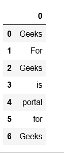
Creating a dataframe using List: DataFrame can be created using a single list or a list of lists.
# import pandas as pdimport pandas as pd# list of stringslst = ['Geeks', 'For', 'Geeks', 'is', 'portal', 'for', 'Geeks']# Calling DataFrame constructor on listdf = pd.DataFrame(lst)print(df) |
Output:
Creating DataFrame from dict of ndarray/lists: To create DataFrame from dict of narray/list, all the narray must be of same length. If index is passed then the length index should be equal to the length of arrays. If no index is passed, then by default, index will be range(n) where n is the array length.
# Python code demonstrate creating # DataFrame from dict narray / lists # By default addresses.import pandas as pd# intialise data of lists.data = {'Name':['Tom', 'nick', 'krish', 'jack'], 'Age':[20, 21, 19, 18]}# Create DataFramedf = pd.DataFrame(data)# Print the output.print(df) |
Output:

For more details refer to Creating a Pandas DataFrame
Dealing with Rows and Columns
A Data frame is a two-dimensional data structure, i.e., data is aligned in a tabular fashion in rows and columns. We can perform basic operations on rows/columns like selecting, deleting, adding, and renaming.
Column Selection: In Order to select a column in Pandas DataFrame, we can either access the columns by calling them by their columns name.
# Import pandas packageimport pandas as pd# Define a dictionary containing employee datadata = {'Name':['Jai', 'Princi', 'Gaurav', 'Anuj'], 'Age':[27, 24, 22, 32], 'Address':['Delhi', 'Kanpur', 'Allahabad', 'Kannauj'], 'Qualification':['Msc', 'MA', 'MCA', 'Phd']}# Convert the dictionary into DataFrame df = pd.DataFrame(data)# select two columnsprint(df[['Name', 'Qualification']]) |
Output:

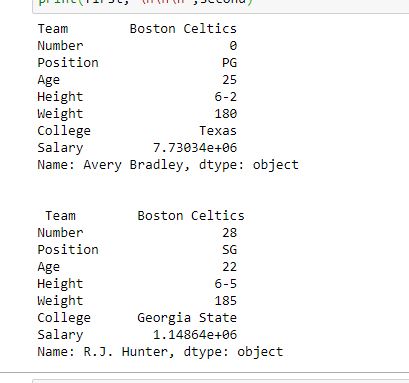
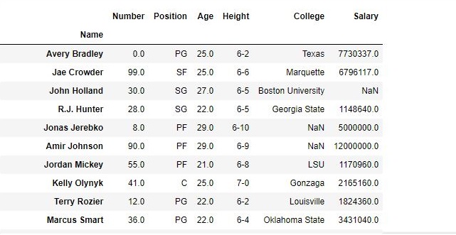
Row Selection: Pandas provide a unique method to retrieve rows from a Data frame. DataFrame.loc[] method is used to retrieve rows from Pandas DataFrame. Rows can also be selected by passing integer location to an iloc[] function.
Note: We’ll be using nba.csv file in below examples.
# importing pandas packageimport pandas as pd# making data frame from csv filedata = pd.read_csv("nba.csv", index_col ="Name")# retrieving row by loc methodfirst = data.loc["Avery Bradley"]second = data.loc["R.J. Hunter"]print(first, "\n\n\n", second) |
Output:
As shown in the output image, two series were returned since there was only one parameter both of the times.
For more Details refer to Dealing with Rows and Columns
Indexing and Selecting Data
Indexing in pandas means simply selecting particular rows and columns of data from a DataFrame. Indexing could mean selecting all the rows and some of the columns, some of the rows and all of the columns, or some of each of the rows and columns. Indexing can also be known as Subset Selection.
Indexing a Dataframe using indexing operator [] :
Indexing operator is used to refer to the square brackets following an object. The .loc and .iloc indexers also use the indexing operator to make selections. In this indexing operator to refer to df[].
Selecting a single columns
In order to select a single column, we simply put the name of the column in-between the brackets
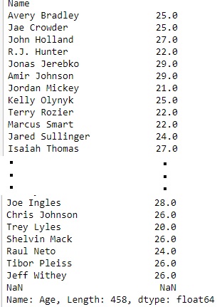
# importing pandas packageimport pandas as pd# making data frame from csv filedata = pd.read_csv("nba.csv", index_col ="Name")# retrieving columns by indexing operatorfirst = data["Age"]print(first) |
Output:
Indexing a DataFrame using .loc[ ] :
This function selects data by the label of the rows and columns. The df.loc indexer selects data in a different way than just the indexing operator. It can select subsets of rows or columns. It can also simultaneously select subsets of rows and columns.
Selecting a single row
In order to select a single row using .loc[], we put a single row label in a .loc function.
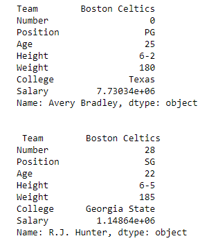
# importing pandas packageimport pandas as pd# making data frame from csv filedata = pd.read_csv("nba.csv", index_col ="Name")# retrieving row by loc methodfirst = data.loc["Avery Bradley"]second = data.loc["R.J. Hunter"]print(first, "\n\n\n", second) |
Output:
As shown in the output image, two series were returned since there was only one parameter both of the times.
Indexing a DataFrame using .iloc[ ] :
This function allows us to retrieve rows and columns by position. In order to do that, we’ll need to specify the positions of the rows that we want, and the positions of the columns that we want as well. The df.iloc indexer is very similar to df.loc but only uses integer locations to make its selections.
Selecting a single row
In order to select a single row using .iloc[], we can pass a single integer to .iloc[] function.
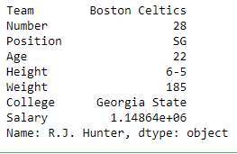
import pandas as pd# making data frame from csv filedata = pd.read_csv("nba.csv", index_col ="Name")# retrieving rows by iloc method row2 = data.iloc[3] print(row2) |
Output:
For more Details refer
Working with Missing Data
Missing Data can occur when no information is provided for one or more items or for a whole unit. Missing Data is a very big problem in real life scenario. Missing Data can also refer to as NA(Not Available) values in pandas.
Checking for missing values using isnull() and notnull() :
In order to check missing values in Pandas DataFrame, we use a function isnull() and notnull(). Both function help in checking whether a value is NaN or not. These function can also be used in Pandas Series in order to find null values in a series.
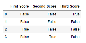
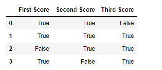
# importing pandas as pdimport pandas as pd# importing numpy as npimport numpy as np# dictionary of listsdict = {'First Score':[100, 90, np.nan, 95], 'Second Score': [30, 45, 56, np.nan], 'Third Score':[np.nan, 40, 80, 98]}# creating a dataframe from listdf = pd.DataFrame(dict)# using isnull() function df.isnull() |
Output:
Filling missing values using fillna(), replace() and interpolate() :
In order to fill null values in a datasets, we use fillna(), replace() and interpolate() function these function replace NaN values with some value of their own. All these function help in filling a null values in datasets of a DataFrame. Interpolate() function is basically used to fill NA values in the dataframe but it uses various interpolation technique to fill the missing values rather than hard-coding the value.
# importing pandas as pdimport pandas as pd# importing numpy as npimport numpy as np# dictionary of listsdict = {'First Score':[100, 90, np.nan, 95], 'Second Score': [30, 45, 56, np.nan], 'Third Score':[np.nan, 40, 80, 98]}# creating a dataframe from dictionarydf = pd.DataFrame(dict)# filling missing value using fillna() df.fillna(0) |
Output:
Dropping missing values using dropna() :
In order to drop a null values from a dataframe, we used dropna() function this fuction drop Rows/Columns of datasets with Null values in different ways.
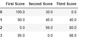
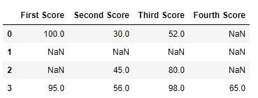
# importing pandas as pdimport pandas as pd# importing numpy as npimport numpy as np# dictionary of listsdict = {'First Score':[100, 90, np.nan, 95], 'Second Score': [30, np.nan, 45, 56], 'Third Score':[52, 40, 80, 98], 'Fourth Score':[np.nan, np.nan, np.nan, 65]}# creating a dataframe from dictionarydf = pd.DataFrame(dict) df |
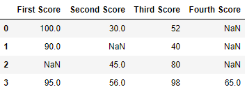
Now we drop rows with at least one Nan value (Null value)
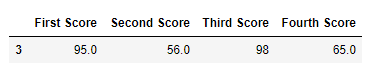
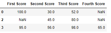
# importing pandas as pdimport pandas as pd# importing numpy as npimport numpy as np# dictionary of listsdict = {'First Score':[100, 90, np.nan, 95], 'Second Score': [30, np.nan, 45, 56], 'Third Score':[52, 40, 80, 98], 'Fourth Score':[np.nan, np.nan, np.nan, 65]}# creating a dataframe from dictionarydf = pd.DataFrame(dict)# using dropna() function df.dropna() |
Output:
For more Details refer to Working with Missing Data in Pandas
Iterating over rows and columns
Iteration is a general term for taking each item of something, one after another. Pandas DataFrame consists of rows and columns so, in order to iterate over dataframe, we have to iterate a dataframe like a dictionary.
Iterating over rows :
In order to iterate over rows, we can use three function iteritems(), iterrows(), itertuples() . These three function will help in iteration over rows.
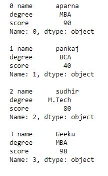
# importing pandas as pdimport pandas as pd # dictionary of listsdict = {'name':["aparna", "pankaj", "sudhir", "Geeku"], 'degree': ["MBA", "BCA", "M.Tech", "MBA"], 'score':[90, 40, 80, 98]}# creating a dataframe from a dictionary df = pd.DataFrame(dict)print(df) |

Now we apply iterrows() function in order to get a each element of rows.
# importing pandas as pdimport pandas as pd # dictionary of listsdict = {'name':["aparna", "pankaj", "sudhir", "Geeku"], 'degree': ["MBA", "BCA", "M.Tech", "MBA"], 'score':[90, 40, 80, 98]}# creating a dataframe from a dictionary df = pd.DataFrame(dict)# iterating over rows using iterrows() function for i, j in df.iterrows(): print(i, j) print() |
Output:
Iterating over Columns :
In order to iterate over columns, we need to create a list of dataframe columns and then iterating through that list to pull out the dataframe columns.
# importing pandas as pdimport pandas as pd # dictionary of listsdict = {'name':["aparna", "pankaj", "sudhir", "Geeku"], 'degree': ["MBA", "BCA", "M.Tech", "MBA"], 'score':[90, 40, 80, 98]} # creating a dataframe from a dictionary df = pd.DataFrame(dict)print(df) |
Now we iterate through columns in order to iterate through columns we first create a list of dataframe columns and then iterate through list.
# creating a list of dataframe columnscolumns = list(df)for i in columns: # printing the third element of the column print (df[i][2]) |
Output:

For more Details refer to Iterating over rows and columns in Pandas DataFrame
DataFrame Methods:
| FUNCTION | DESCRIPTION |
|---|---|
| index() | Method returns index (row labels) of the DataFrame |
| insert() | Method inserts a column into a DataFrame |
| add() | Method returns addition of dataframe and other, element-wise (binary operator add) |
| sub() | Method returns subtraction of dataframe and other, element-wise (binary operator sub) |
| mul() | Method returns multiplication of dataframe and other, element-wise (binary operator mul) |
| div() | Method returns floating division of dataframe and other, element-wise (binary operator truediv) |
| unique() | Method extracts the unique values in the dataframe |
| nunique() | Method returns count of the unique values in the dataframe |
| value_counts() | Method counts the number of times each unique value occurs within the Series |
| columns() | Method returns the column labels of the DataFrame |
| axes() | Method returns a list representing the axes of the DataFrame |
| isnull() | Method creates a Boolean Series for extracting rows with null values |
| notnull() | Method creates a Boolean Series for extracting rows with non-null values |
| between() | Method extracts rows where a column value falls in between a predefined range |
| isin() | Method extracts rows from a DataFrame where a column value exists in a predefined collection |
| dtypes() | Method returns a Series with the data type of each column. The result’s index is the original DataFrame’s columns |
| astype() | Method converts the data types in a Series |
| values() | Method returns a Numpy representation of the DataFrame i.e. only the values in the DataFrame will be returned, the axes labels will be removed |
| sort_values()- Set1, Set2 | Method sorts a data frame in Ascending or Descending order of passed Column |
| sort_index() | Method sorts the values in a DataFrame based on their index positions or labels instead of their values but sometimes a data frame is made out of two or more data frames and hence later index can be changed using this method |
| loc[] | Method retrieves rows based on index label |
| iloc[] | Method retrieves rows based on index position |
| ix[] | Method retrieves DataFrame rows based on either index label or index position. This method combines the best features of the .loc[] and .iloc[] methods |
| rename() | Method is called on a DataFrame to change the names of the index labels or column names |
| columns() | Method is an alternative attribute to change the coloumn name |
| drop() | Method is used to delete rows or columns from a DataFrame |
| pop() | Method is used to delete rows or columns from a DataFrame |
| sample() | Method pulls out a random sample of rows or columns from a DataFrame |
| nsmallest() | Method pulls out the rows with the smallest values in a column |
| nlargest() | Method pulls out the rows with the largest values in a column |
| shape() | Method returns a tuple representing the dimensionality of the DataFrame |
| ndim() | Method returns an ‘int’ representing the number of axes / array dimensions. Returns 1 if Series, otherwise returns 2 if DataFrame |
| dropna() | Method allows the user to analyze and drop Rows/Columns with Null values in different ways |
| fillna() | Method manages and let the user replace NaN values with some value of their own |
| rank() | Values in a Series can be ranked in order with this method |
| query() | Method is an alternate string-based syntax for extracting a subset from a DataFrame |
| copy() | Method creates an independent copy of a pandas object |
| duplicated() | Method creates a Boolean Series and uses it to extract rows that have duplicate values |
| drop_duplicates() | Method is an alternative option to identifying duplicate rows and removing them through filtering |
| set_index() | Method sets the DataFrame index (row labels) using one or more existing columns |
| reset_index() | Method resets index of a Data Frame. This method sets a list of integer ranging from 0 to length of data as index |
| where() | Method is used to check a Data Frame for one or more condition and return the result accordingly. By default, the rows not satisfying the condition are filled with NaN value |
##################################
import os
import pandas as pd
#1: Import the excel file and call it xls_file
excel_file = pd.ExcelFile('enquiries.xls')
#2. View the excel_file's sheet names
print(excel_file.sheet_names)
#3 : Read an excel file using read_excel() method of pandas.
# read by default 1st sheet of an excel file
dataframe1 = pd.read_excel('enquiries.xls')
print(dataframe1)
#4. read 2nd sheet of an excel file replace missing values with nan
# By default Python treats blank values as NAN
# To treat any other garbage values like '??', "?????" we need to instruct using paramaetr na_values
#dataframe2 = pd.read_excel('enquiries.xls', sheet_name = 1,na_values=["??","????"])
# Type casting a column
5. dataframe2 ["Name]"= dataframe2 ["Name]".astype("object")
# total bytes by the column
5. dataframe2 ["Name]"= dataframe2 ["Name]".nbytes
# Replace One word with value under col 'Name'
5. dataframe2 ["Name]".replace('one',1,inplace=true)
# total no of null values in a data frame
5. dataframe2.isnull.sum()
#7 Access each value in a column using loop
l=df['age']
print(len(l))
for i in range(len(l)):
print(df['age'][i])
#8 append new column and find each age is adult or not
df.insert(2,"adult","")
# Access each value in a column using loop and
l=df['age']
print(len(l))
for i in range(len(l)):
print(df['age'][i])
if (df['age'][i] < 20):
df['adult'][i] ='yes'
else:
df['adult'][i] ='no'
# Find all values under column age
l=df['age'].get_values()
print(l)
# Find total unique values under column age
l=df['age'].value_counts()
print(l)
# Function on col to create new col uwith updated values i.e ages using function
#Create new column
df.insert(2,"new age","")
def incr_age(v):
return v+2
df['new age']=incr_age(df['age'])
print(df)
#4. read 2nd sheet of an excel file
#dataframe2 = pd.read_excel('enquiries.xls', sheet_name = 1,)
#5 : Read an excel file using read_excel() method of pandas.
db=pd.read_excel("enquiries.xls",sheet_name="Python")
#print(db)
#6: Load the excel_file's Sheet1 as a dataframe
df = excel_file.parse('Python')
print(df)
require_cols = [2]
#7. only read specific columns from an excel file
required_df = pd.read_excel('enquiries.xls', usecols = require_cols)
print(required_df)
#8 Handling missing data using 'na_values' parameter of the read_excel() method.
dataframe = pd.read_excel('enquiries.xls', na_values = "Missing",
sheet_name = "Python")
print(dataframe)
#9 : Skip starting rows when Reading an Excel File using 'skiprows' parameter of read_excel() method.
df = pd.read_excel('enquiries.xls', sheet_name = "Python", skiprows = 2)
print(df)
#10 #6 : Set the header to any row and start reading from that row, using 'header' parameter of the read_excel() method.
# setting the 3rd row as header.
df = pd.read_excel('enquiries.xls', sheet_name = "Python", header = 2)
print(df)
#11 : Reading Multiple Excel Sheets using 'sheet_name' parameter of the read_excel()method.
# read both 1st and 2nd sheet.
df = pd.read_excel('enquiries.xls', na_values = "Mssing", sheet_name =[0, 1])
print(df)
#12 Reading all Sheets of the excel file together using 'sheet_name' parameter of the read_excel() method.
# read all sheets together.
all_sheets_df = pd.read_excel('enquiries.xls', na_values = "Missing",
sheet_name = None)
print(all_sheets_df)
#13 retrieving columns by indexing operator
df = pd.read_excel('enquiries.xls', na_values = "Mssing", sheet_name ="Python")
print(df)
first = df["Mob Num"]
print(first)
# 14 Shallow caopy
df2=df
print(df2)
df3=df.copy(deep=False)
print(df3)
# 15 Deep copy
df3=df.copy(deep=True)
print(df3)
#16 Get Row labels
print(df3.index)
#17 Get columns labels
print(df3.columns)
#18 Get columns labels
print(df3.size)
#19 Get columns labels
print(df3.shape)
#20 Get memory usage
print(df3.memory_usage)
#21 Get first 5 rows
print(df3.head(5))
#22 Get lst 5 rows
print(df3.tail(5))
#23 Indexing row=integer and column=label name
#Arshia.Shaik
#Value at row 4 and column "Name"
print(df3.at[4,"Name"])
#23 Indexing row=integer and column=label name
#Arshia.Shaik
#Value at row 4 and column "Name"
print(df3.iat[4,1])
#24 Indexing group of rows and columns
#all rows with only column="Name"
#Arshia.Shaik
#Value at row 4 and column "Name"
print(df3.loc[:,"Name"])
print(df3.loc[[900,901],["Name","E.mail"]])
Exploratory Data Analysis in Python
What is Exploratory Data Analysis (EDA) ?
EDA is a phenomenon under data analysis used for gaining a better understanding of data aspects like:
– main features of data
– variables and relationships that hold between them
– identifying which variables are important for our problem
We shall look at various exploratory data analysis methods like:
- Descriptive Statistics, which is a way of giving a brief overview of the dataset we are dealing with, including some measures and features of the sample
- Grouping data [Basic grouping with group by]
- ANOVA, Analysis Of Variance, which is a computational method to divide variations in an observations set into different components.
- Correlation and correlation methods
The dataset we’ll be using is chile voting dataset, which you can import in python as:
import pandas as pd |
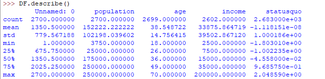
Descriptive Statistics
Descriptive statistics is a helpful way to understand characteristics of your data and to get a quick summary of it. Pandas in python provide an interesting method describe(). The describe function applies basic statistical computations on the dataset like extreme values, count of data points standard deviation etc. Any missing value or NaN value is automatically skipped. describe() function gives a good picture of distribution of data.
DF.describe() |
Here’s the output you’ll get on running above code:
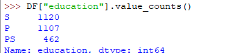
Another useful method if value_counts() which can get count of each category in a categorical attributed series of values. For an instance suppose you are dealing with a dataset of customers who are divided as youth, medium and old categories under column name age and your dataframe is “DF”. You can run this statement to know how many people fall in respective categories. In our data set example education column can be used
DF["education"].value_counts() |
The output of the above code will be:
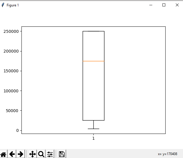
One more useful tool is boxplot which you can use through matplotlib module. Boxplot is a pictorial representation of distribution of data which shows extreme values, median and quartiles. We can easily figure out outliers by using boxplots. Now consider the dataset we’ve been dealing with again and lets draw a boxplot on attribute population
import pandas as pd import matplotlib.pyplot as plt DF = pd.read_csv("https://raw.githubusercontent.com / fivethirtyeight / data / master / airline-safety / airline-safety.csv") y = list(DF.population) plt.boxplot(y) plt.show() |
The output plot would look like this with spotting out outliers:
Grouping data
Group by is an interesting measure available in pandas which can help us figure out effect of different categorical attributes on other data variables. Let’s see an example on the same dataset where we want to figure out affect of people’s age and education on the voting dataset.
DF.groupby(['education', 'vote']).mean() |
The output would be somewhat like this:
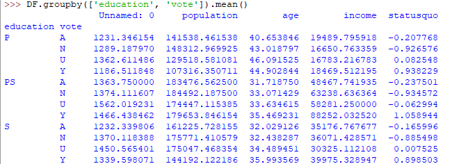
If this group by output table is less understandable further analysts use pivot tables and heat maps for visualization on them.
ANOVA
ANOVA stands for Analysis of Variance. It is performed to figure out the relation between the different group of categorical data.
Under ANOVA we have two measures as result:
– F-testscore : which shows the variaton of groups mean over variation
– p-value: it shows the importance of the result
This can be performed using python module scipy method name f_oneway()
Syntax:
import scipy.stats as st
st.f_oneway(sample1, sample2, ..)
These samples are sample measurements for each group.
As a conclusion, we can say that there is a strong correlation between other variables and a categorical variable if the ANOVA test gives us a large F-test value and a small p-value.
Correlation and Correlation computation
Correlation is a simple relationship between two variables in a context such that one variable affects the other. Correlation is different from act of causing. One way to calculate correlation among variables is to find Pearson correlation. Here we find two parameters namely, Pearson coefficient and p-value. We can say there is a strong correlation between two variables when Pearson correlation coefficient is close to either 1 or -1 and the p-value is less than 0.0001.
Scipy module also provides a method to perform pearson correlation analysis, syntax:
Exploratory Data Analysis in Python | Set 1
Exploratory Data Analysis is a technique to analyze data with visual techniques and all statistical results. We will learn about how to apply these techniques before applying any Machine Learning Models.
To get the link to csv file used, click here.
Loading Libraries:
import numpy as np import pandas as pd import seaborn as sns import matplotlib.pyplot as plt from scipy.stats import trim_mean |
Loading Data:
data = pd.read_csv("state.csv") # Check the type of data print ("Type : ", type(data), "\n\n") # Printing Top 10 Records print ("Head -- \n", data.head(10)) # Printing last 10 Records print ("\n\n Tail -- \n", data.tail(10)) |
Output :
Type : class 'pandas.core.frame.DataFrame'


Head --
          State  Population  Murder.Rate Abbreviation
0      Alabama     4779736          5.7           AL
1       Alaska      710231          5.6           AK
2      Arizona     6392017          4.7           AZ
3     Arkansas     2915918          5.6           AR
4   California    37253956          4.4           CA
5     Colorado     5029196          2.8           CO
6  Connecticut     3574097          2.4           CT
7     Delaware      897934          5.8           DE
8      Florida    18801310          5.8           FL
9      Georgia     9687653          5.7           GA


 Tail --
             State  Population  Murder.Rate Abbreviation
40   South Dakota      814180          2.3           SD
41      Tennessee     6346105          5.7           TN
42          Texas    25145561          4.4           TX
43           Utah     2763885          2.3           UT
44        Vermont      625741          1.6           VT
45       Virginia     8001024          4.1           VA
46     Washington     6724540          2.5           WA
47  West Virginia     1852994          4.0           WV
48      Wisconsin     5686986          2.9           WI
49        Wyoming      563626          2.7           WY
Code #1 : Adding Column to the dataframe
# Adding a new column with derived data data['PopulationInMillions'] = data['Population']/1000000 # Changed data print (data.head(5)) |
Output :
        State  Population  Murder.Rate Abbreviation  PopulationInMillions
0     Alabama     4779736          5.7           AL              4.779736
1      Alaska      710231          5.6           AK              0.710231
2     Arizona     6392017          4.7           AZ              6.392017
3    Arkansas     2915918          5.6           AR              2.915918
4  California    37253956          4.4           CA             37.253956
Code #2 : Data Description
data.describe() |
Output :

Code #3 : Data Info
data.info() |
Output :
RangeIndex: 50 entries, 0 to 49
Data columns (total 4 columns):
State           50 non-null object
Population      50 non-null int64
Murder.Rate     50 non-null float64
Abbreviation    50 non-null object
dtypes: float64(1), int64(1), object(2)
memory usage: 1.6+ KB
Code #4 : Renaming a column heading
# Rename column heading as it # has '.' in it which will create # problems when dealing functions data.rename(columns ={'Murder.Rate': 'MurderRate'}, inplace = True) # Lets check the column headings list(data) |
Output :
['State', 'Population', 'MurderRate', 'Abbreviation']
Code #5 : Calculating Mean
Population_mean = data.Population.mean() print ("Population Mean : ", Population_mean) MurderRate_mean = data.MurderRate.mean() print ("\nMurderRate Mean : ", MurderRate_mean) |
Output:
Population Mean :  6162876.3

MurderRate Mean :  4.066
Code #6 : Trimmed mean
# Mean after discarding top and # bottom 10 % values eliminating outliers population_TM = trim_mean(data.Population, 0.1) print ("Population trimmed mean: ", population_TM) murder_TM = trim_mean(data.MurderRate, 0.1) print ("\nMurderRate trimmed mean: ", murder_TM) |
Output :
Population trimmed mean:  4783697.125

MurderRate trimmed mean:  3.9450000000000003
Code #7 : Weighted Mean
# here murder rate is weighed as per # the state population murderRate_WM = np.average(data.MurderRate, weights = data.Population) print ("Weighted MurderRate Mean: ", murderRate_WM) |
Output :
Weighted MurderRate Mean: 4.445833981123393
Code #8 : Median
Population_median = data.Population.median() print ("Population median : ", Population_median) MurderRate_median = data.MurderRate.median() print ("\nMurderRate median : ", MurderRate_median) |
Output :
Population median :  4436369.5

MurderRate median :  4.0
Exploratory Data Analysis in Python | Set 2
In the previous article, we have discussed some basic techniques to analyze the data, now let’s see the visual techniques.
Let’s see the basic techniques –
# Loading Libraries import numpy as np import pandas as pd import seaborn as sns import matplotlib.pyplot as plt from scipy.stats import trim_mean # Loading Data data = pd.read_csv("state.csv") # Check the type of data print ("Type : ", type(data), "\n\n") # Printing Top 10 Records print ("Head -- \n", data.head(10)) # Printing last 10 Records print ("\n\n Tail -- \n", data.tail(10)) # Adding a new column with derived data data['PopulationInMillions'] = data['Population']/1000000 # Changed data print (data.head(5)) # Rename column heading as it # has '.' in it which will create # problems when dealing functions data.rename(columns ={'Murder.Rate': 'MurderRate'}, inplace = True) # Lets check the column headings list(data) |
Output :
Type : class 'pandas.core.frame.DataFrame'


Head --
          State  Population  Murder.Rate Abbreviation
0      Alabama     4779736          5.7           AL
1       Alaska      710231          5.6           AK
2      Arizona     6392017          4.7           AZ
3     Arkansas     2915918          5.6           AR
4   California    37253956          4.4           CA
5     Colorado     5029196          2.8           CO
6  Connecticut     3574097          2.4           CT
7     Delaware      897934          5.8           DE
8      Florida    18801310          5.8           FL
9      Georgia     9687653          5.7           GA


 Tail --
             State  Population  Murder.Rate Abbreviation
40   South Dakota      814180          2.3           SD
41      Tennessee     6346105          5.7           TN
42          Texas    25145561          4.4           TX
43           Utah     2763885          2.3           UT
44        Vermont      625741          1.6           VT
45       Virginia     8001024          4.1           VA
46     Washington     6724540          2.5           WA
47  West Virginia     1852994          4.0           WV
48      Wisconsin     5686986          2.9           WI
49        Wyoming      563626          2.7           WY


        State  Population  Murder.Rate Abbreviation  PopulationInMillions
0     Alabama     4779736          5.7           AL              4.779736
1      Alaska      710231          5.6           AK              0.710231
2     Arizona     6392017          4.7           AZ              6.392017
3    Arkansas     2915918          5.6           AR              2.915918
4  California    37253956          4.4           CA             37.253956


['State', 'Population', 'MurderRate', 'Abbreviation']
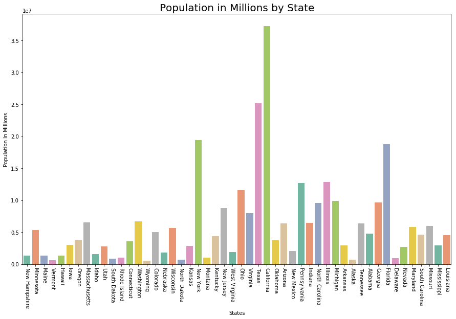
Visualizing Population per Million
# Plot Population In Millions fig, ax1 = plt.subplots() fig.set_size_inches(15, 9) ax1 = sns.barplot(x ="State", y ="Population", data = data.sort_values('MurderRate'), palette ="Set2") ax1.set(xlabel ='States', ylabel ='Population In Millions') ax1.set_title('Population in Millions by State', size = 20) plt.xticks(rotation =-90) |
Output:
(array([ 0,  1,  2,  3,  4,  5,  6,  7,  8,  9, 10, 11, 12, 13, 14, 15, 16,
        17, 18, 19, 20, 21, 22, 23, 24, 25, 26, 27, 28, 29, 30, 31, 32, 33,
        34, 35, 36, 37, 38, 39, 40, 41, 42, 43, 44, 45, 46, 47, 48, 49]),
 a list of 50 Text xticklabel objects)
Visualizing Murder Rate per Lakh
# Plot Murder Rate per 1, 00, 000 fig, ax2 = plt.subplots() fig.set_size_inches(15, 9) ax2 = sns.barplot( x ="State", y ="MurderRate", data = data.sort_values('MurderRate', ascending = 1), palette ="husl") ax2.set(xlabel ='States', ylabel ='Murder Rate per 100000') ax2.set_title('Murder Rate by State', size = 20) plt.xticks(rotation =-90) |
Output :
(array([ 0,  1,  2,  3,  4,  5,  6,  7,  8,  9, 10, 11, 12, 13, 14, 15, 16,
        17, 18, 19, 20, 21, 22, 23, 24, 25, 26, 27, 28, 29, 30, 31, 32, 33,
        34, 35, 36, 37, 38, 39, 40, 41, 42, 43, 44, 45, 46, 47, 48, 49]),
 a list of 50 Text xticklabel objects)
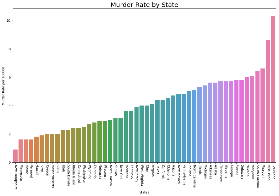
Although Louisiana is ranked 17 by population (about 4.53M), it has the highest Murder rate of 10.3 per 1M people.
Code #1 : Standard Deviation
Population_std = data.Population.std() print ("Population std : ", Population_std) MurderRate_std = data.MurderRate.std() print ("\nMurderRate std : ", MurderRate_std) |
Output :
Population std :  6848235.347401142

MurderRate std :  1.915736124302923
Code #2 : Variance
Population_var = data.Population.var() print ("Population var : ", Population_var) MurderRate_var = data.MurderRate.var() print ("\nMurderRate var : ", MurderRate_var) |
Output :
Population var :  46898327373394.445

MurderRate var :  3.670044897959184
Code #3 : Inter Quartile Range
# Inter Quartile Range of Population population_IQR = data.Population.describe()['75 %'] - data.Population.describe()['25 %'] print ("Population IQR : ", population_IRQ) # Inter Quartile Range of Murder Rate MurderRate_IQR = data.MurderRate.describe()['75 %'] - data.MurderRate.describe()['25 %'] print ("\nMurderRate IQR : ", MurderRate_IQR) |
Output :
Population IQR :  4847308.0

MurderRate IQR :  3.124999999999999
Code #4 : Median Absolute Deviation (MAD)
Population_mad = data.Population.mad() print ("Population mad : ", Population_mad) MurderRate_mad = data.MurderRate.mad() print ("\nMurderRate mad : ", MurderRate_mad) |
Output :
Population mad :  4450933.356000001

MurderRate mad :  1.5526400000000005
Python | Math operations for Data analysis
Python is a great language for doing data analysis, primarily because of the fantastic ecosystem of data-centric Python packages. Pandas is one of those packages, and makes importing and analyzing data much easier.
There are some important math operations that can be performed on a pandas series to simplify data analysis using Python and save a lot of time.
To get the data-set used, click here.
s=read_csv("stock.csv", squeeze=True)
#reading csv file and making seires
| FUNCTION | USE |
|---|---|
| s.sum() | Returns sum of all values in the series |
| s.mean() | Returns mean of all values in series. Equals to s.sum()/s.count()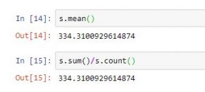 |
| s.std() | Returns standard deviation of all values |
| s.min() or s.max() | Return min and max values from series |
| s.idxmin() or s.idxmax() | Returns index of min or max value in series |
| s.median() | Returns median of all value |
| s.mode() | Returns mode of the series |
| s.value_counts() | Returns series with frequency of each value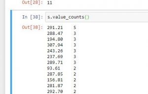 |
| s.describe() | Returns a series with information like mean, mode etc depending on dtype of data passed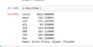 |
Code #1:
# import pandas for reading csv file import pandas as pd #reading csv file s = pd.read_csv("stock.csv", squeeze = True) #using count function print(s.count()) #using sum function print(s.sum()) #using mean function print(s.mean()) #calculatin average print(s.sum()/s.count()) #using std function print(s.std()) #using min function print(s.min()) #using max function print(s.max()) #using count function print(s.median()) #using mode function print(s.mode()) |
Output:
3012
1006942.0
334.3100929614874
334.3100929614874
173.18720477113115
49.95
782.22
283.315
0    291.21
Code #2:
# import pandas for reading csv file import pandas as pd #reading csv file s = pd.read_csv("stock.csv", squeeze = True) #using describe function print(s.describe()) #using count function print(s.idxmax()) #using idxmin function print(s.idxmin()) #count of elements having value 3 print(s.value_counts().head(3)) |
Output:
dtype: float64
count    3012.000000
mean      334.310093
std       173.187205
min        49.950000
25%       218.045000
50%       283.315000
75%       443.000000
max       782.220000
Name: Stock Price, dtype: float64

3011
11
291.21    5
288.47    3
194.80    3
Name: Stock Price, dtype: int64
Unexpected Outputs and Restrictions:
-
- .sum(), .mean(), .mode(), .median() and other such mathematical operations are not applicable on string or any other data type than numeric value.
- .sum() on a string series would give an unexpected output and return a string by concatenating every string.
Working with Missing Data in Pandas
Missing Data can occur when no information is provided for one or more items or for a whole unit. Missing Data is a very big problem in real life scenario. Missing Data can also refer to as NA(Not Available) values in pandas. In DataFrame sometimes many datasets simply arrive with missing data, either because it exists and was not collected or it never existed. For Example, Suppose different user being surveyed may choose not to share their income, some user may choose not to share the address in this way many datasets went missing.

In Pandas missing data is represented by two value:
- None: None is a Python singleton object that is often used for missing data in Python code.
- NaN : NaN (an acronym for Not a Number), is a special floating-point value recognized by all systems that use the standard IEEE floating-point representation
Pandas treat None and NaN as essentially interchangeable for indicating missing or null values. To facilitate this convention, there are several useful functions for detecting, removing, and replacing null values in Pandas DataFrame :
In this article we are using CSV file, to download the CSV file used, Click Here.
Checking for missing values using isnull() and notnull()
In order to check missing values in Pandas DataFrame, we use a function isnull() and notnull(). Both function help in checking whether a value is NaN or not. These function can also be used in Pandas Series in order to find null values in a series.
Checking for missing values using isnull()
In order to check null values in Pandas DataFrame, we use isnull() function this function return dataframe of Boolean values which are True for NaN values.
Code #1:
# importing pandas as pd import pandas as pd # importing numpy as np import numpy as np # dictionary of lists dict = {'First Score':[100, 90, np.nan, 95], 'Second Score': [30, 45, 56, np.nan], 'Third Score':[np.nan, 40, 80, 98]} # creating a dataframe from list df = pd.DataFrame(dict) # using isnull() function df.isnull() |
Output:
Code #2:
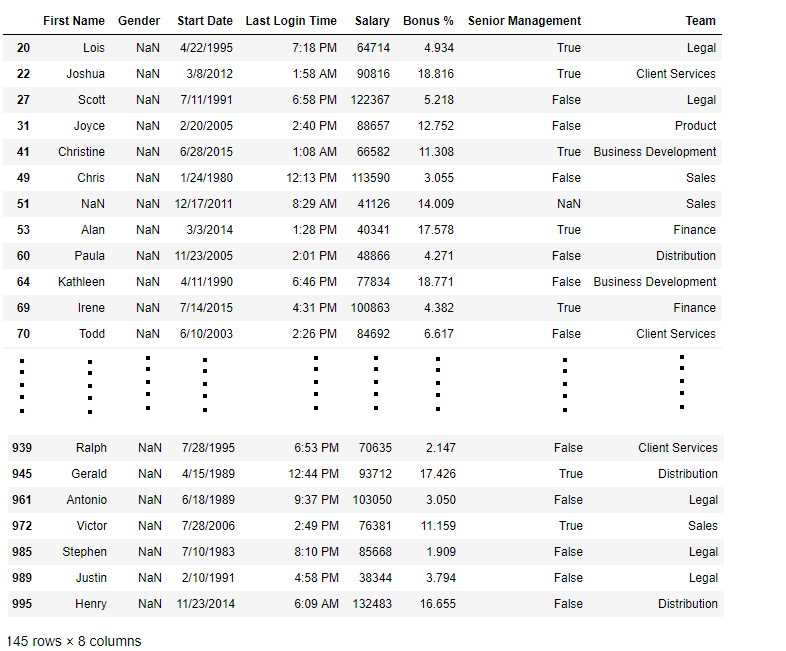
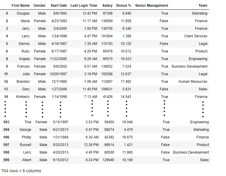
# importing pandas package import pandas as pd # making data frame from csv file data = pd.read_csv("employees.csv") # creating bool series True for NaN values bool_series = pd.isnull(data["Gender"]) # filtering data # displaying data only with Gender = NaN data[bool_series] |
Output:
As shown in the output image, only the rows having Gender = NULL are displayed.
Checking for missing values using notnull()
In order to check null values in Pandas Dataframe, we use notnull() function this function return dataframe of Boolean values which are False for NaN values.
Code #3:
# importing pandas as pd import pandas as pd # importing numpy as np import numpy as np # dictionary of lists dict = {'First Score':[100, 90, np.nan, 95], 'Second Score': [30, 45, 56, np.nan], 'Third Score':[np.nan, 40, 80, 98]} # creating a dataframe using dictionary df = pd.DataFrame(dict) # using notnull() function df.notnull() |
Output:
Code #4:
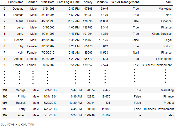
# importing pandas package import pandas as pd # making data frame from csv file data = pd.read_csv("employees.csv") # creating bool series True for NaN values bool_series = pd.notnull(data["Gender"]) # filtering data # displayind data only with Gender = Not NaN data[bool_series] |
Output:
As shown in the output image, only the rows having Gender = NOT NULL are displayed.
Filling missing values using fillna(), replace() and interpolate()
In order to fill null values in a datasets, we use fillna(), replace() and interpolate() function these function replace NaN values with some value of their own. All these function help in filling a null values in datasets of a DataFrame. Interpolate() function is basically used to fill NA values in the dataframe but it uses various interpolation technique to fill the missing values rather than hard-coding the value.
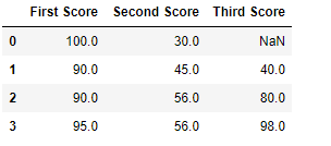
Code #1: Filling null values with a single value
# importing pandas as pd import pandas as pd # importing numpy as np import numpy as np # dictionary of lists dict = {'First Score':[100, 90, np.nan, 95], 'Second Score': [30, 45, 56, np.nan], 'Third Score':[np.nan, 40, 80, 98]} # creating a dataframe from dictionary df = pd.DataFrame(dict) # filling missing value using fillna() df.fillna(0) |
Output:
Code #2: Filling null values with the previous ones
# importing pandas as pd import pandas as pd # importing numpy as np import numpy as np # dictionary of lists dict = {'First Score':[100, 90, np.nan, 95], 'Second Score': [30, 45, 56, np.nan], 'Third Score':[np.nan, 40, 80, 98]} # creating a dataframe from dictionary df = pd.DataFrame(dict) # filling a missing value with # previous ones df.fillna(method ='pad') |
Output:
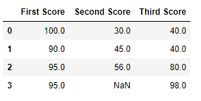
Code #3: Filling null value with the next ones
# importing pandas as pd import pandas as pd # importing numpy as np import numpy as np # dictionary of lists dict = {'First Score':[100, 90, np.nan, 95], 'Second Score': [30, 45, 56, np.nan], 'Third Score':[np.nan, 40, 80, 98]} # creating a dataframe from dictionary df = pd.DataFrame(dict) # filling null value using fillna() function df.fillna(method ='bfill') |
Output:
Code #4: Filling null values in CSV File
# importing pandas package import pandas as pd # making data frame from csv file data = pd.read_csv("employees.csv") # Printing the first 10 to 24 rows of # the data frame for visualization data[10:25] |
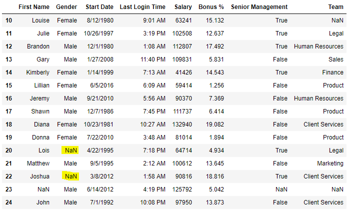
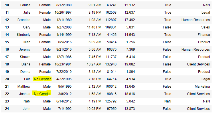
Now we are going to fill all the null values in Gender column with “No Gender”
# importing pandas package import pandas as pd # making data frame from csv file data = pd.read_csv("employees.csv") # filling a null values using fillna() data["Gender"].fillna("No Gender", inplace = True) data |
Output:
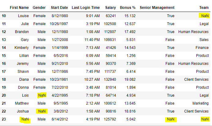
Code #5: Filling a null values using replace() method
# importing pandas package import pandas as pd # making data frame from csv file data = pd.read_csv("employees.csv") # Printing the first 10 to 24 rows of # the data frame for visualization data[10:25] |
Output:
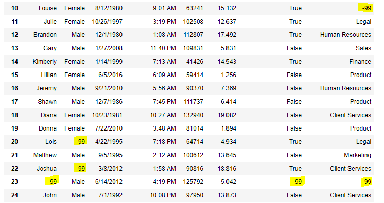
Now we are going to replace the all Nan value in the data frame with -99 value.
# importing pandas package import pandas as pd # making data frame from csv file data = pd.read_csv("employees.csv") # will replace Nan value in dataframe with value -99 data.replace(to_replace = np.nan, value = -99) |
Output:
Code #6: Using interpolate() function to fill the missing values using linear method.
# importing pandas as pd import pandas as pd # Creating the dataframe df = pd.DataFrame({"A":[12, 4, 5, None, 1], "B":[None, 2, 54, 3, None], "C":[20, 16, None, 3, 8], "D":[14, 3, None, None, 6]}) # Print the dataframe df |
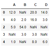
Let’s interpolate the missing values using Linear method. Note that Linear method ignore the index and treat the values as equally spaced.
# to interpolate the missing values df.interpolate(method ='linear', limit_direction ='forward') |
Output:
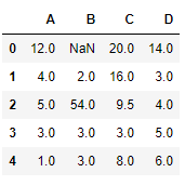
As we can see the output, values in the first row could not get filled as the direction of filling of values is forward and there is no previous value which could have been used in interpolation.
Dropping missing values using dropna()
In order to drop a null values from a dataframe, we used dropna() function this fuction drop Rows/Columns of datasets with Null values in different ways.
Code #1: Dropping rows with at least 1 null value.
# importing pandas as pd import pandas as pd # importing numpy as np import numpy as np # dictionary of lists dict = {'First Score':[100, 90, np.nan, 95], 'Second Score': [30, np.nan, 45, 56], 'Third Score':[52, 40, 80, 98], 'Fourth Score':[np.nan, np.nan, np.nan, 65]} # creating a dataframe from dictionary df = pd.DataFrame(dict) df |
Now we drop rows with at least one Nan value (Null value)
# importing pandas as pd import pandas as pd # importing numpy as np import numpy as np # dictionary of lists dict = {'First Score':[100, 90, np.nan, 95], 'Second Score': [30, np.nan, 45, 56], 'Third Score':[52, 40, 80, 98], 'Fourth Score':[np.nan, np.nan, np.nan, 65]} # creating a dataframe from dictionary df = pd.DataFrame(dict) # using dropna() function df.dropna() |
Output:
Code #2: Dropping rows if all values in that row are missing.
# importing pandas as pd import pandas as pd # importing numpy as np import numpy as np # dictionary of lists dict = {'First Score':[100, np.nan, np.nan, 95], 'Second Score': [30, np.nan, 45, 56], 'Third Score':[52, np.nan, 80, 98], 'Fourth Score':[np.nan, np.nan, np.nan, 65]} # creating a dataframe from dictionary df = pd.DataFrame(dict) df |
Now we drop a rows whose all data is missing or contain null values(NaN)
# importing pandas as pd import pandas as pd # importing numpy as np import numpy as np # dictionary of lists dict = {'First Score':[100, np.nan, np.nan, 95], 'Second Score': [30, np.nan, 45, 56], 'Third Score':[52, np.nan, 80, 98], 'Fourth Score':[np.nan, np.nan, np.nan, 65]} df = pd.DataFrame(dict) # using dropna() function df.dropna(how = 'all') |
Output:
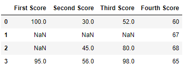
Code #3: Dropping columns with at least 1 null value.
# importing pandas as pd import pandas as pd # importing numpy as np import numpy as np # dictionary of lists dict = {'First Score':[100, np.nan, np.nan, 95], 'Second Score': [30, np.nan, 45, 56], 'Third Score':[52, np.nan, 80, 98], 'Fourth Score':[60, 67, 68, 65]} # creating a dataframe from dictionary df = pd.DataFrame(dict) df |
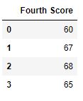
Now we drop a columns which have at least 1 missing values
# importing pandas as pd import pandas as pd # importing numpy as np import numpy as np # dictionary of lists dict = {'First Score':[100, np.nan, np.nan, 95], 'Second Score': [30, np.nan, 45, 56], 'Third Score':[52, np.nan, 80, 98], 'Fourth Score':[60, 67, 68, 65]} # creating a dataframe from dictionary df = pd.DataFrame(dict) # using dropna() function df.dropna(axis = 1) |
Output :
Code #4: Dropping Rows with at least 1 null value in CSV file
# importing pandas module import pandas as pd # making data frame from csv file data = pd.read_csv("employees.csv") # making new data frame with dropped NA values new_data = data.dropna(axis = 0, how ='any') new_data |
Output:
Now we compare sizes of data frames so that we can come to know how many rows had at least 1 Null value
print("Old data frame length:", len(data)) print("New data frame length:", len(new_data)) print("Number of rows with at least 1 NA value: ", (len(data)-len(new_data))) |
Output :
Old data frame length: 1000
New data frame length: 764
Number of rows with at least 1 NA value:  236
Since the difference is 236, there were 236 rows which had at least 1 Null value in any column.
#################### MISSING VALUES########################
# Dictionary
df=pd.DataFrame({'name':['a','b','a'],'age':[21,20,32]},index=["one","two","three"])
print(df)
# Is there any nan(not a number) values i.e blank
# returns data frame of boolean values
print(df.isna())
## Is there any nan values i.e blank
print(df.isnull())
# count the total nan values against eash column
print(df.isna().sum())
#count the total nan values against eash column
print(df.isnull().sum())
#Sub setting the rows that have one or more missing values
missing=df[df.isnull().any(axis=1)]
# Statistical details about the frame
# for each col, mean, median, etc
print(df.describe())
# To get mean of column
print(df['age'].mean())
# To fill missing value with mean in the col 'age'
#fillna() fills the missed values
df['age'].fillna(df['age'].mean(),inplace=True)
# returns a series labelled 1d array
# How many times each unique value is repated
print(df['name'].value_counts())
# To access first item in the series
print(df['name'].value_counts().index[0])
df['name'].fillna(df['name'].value_counts().index[0],inplace=True)
######
Python | Pandas DataFrame.dtypes
Pandas DataFrame is a two-dimensional size-mutable, potentially heterogeneous tabular data structure with labeled axes (rows and columns). Arithmetic operations align on both row and column labels. It can be thought of as a dict-like container for Series objects. This is the primary data structure of the Pandas.
Pandas DataFrame.dtypes attribute return the dtypes in the DataFrame. It returns a Series with the data type of each column.
Syntax: DataFrame.dtypes
Parameter : None
Returns : dtype of each column
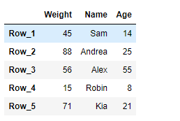
Example #1: Use DataFrame.dtypes attribute to find out the data type (dtype) of each column in the given dataframe.
# importing pandas as pd import pandas as pd # Creating the DataFrame df = pd.DataFrame({'Weight':[45, 88, 56, 15, 71], 'Name':['Sam', 'Andrea', 'Alex', 'Robin', 'Kia'], 'Age':[14, 25, 55, 8, 21]}) # Create the index index_ = ['Row_1', 'Row_2', 'Row_3', 'Row_4', 'Row_5'] # Set the index df.index = index_ # Print the DataFrame print(df) |
Output :
Now we will use DataFrame.dtypes attribute to find out the data type of each column in the given dataframe.
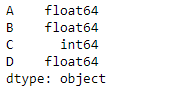
# return the dtype of each column result = df.dtypes # Print the result print(result) |
Output :
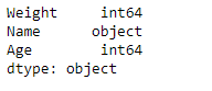
As we can see in the output, the DataFrame.dtypes attribute has successfully returned the data types of each column in the given dataframe.
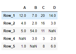
Example #2: Use DataFrame.dtypes attribute to find out the data type (dtype) of each column in the given dataframe.
# importing pandas as pd import pandas as pd # Creating the DataFrame df = pd.DataFrame({"A":[12, 4, 5, None, 1], "B":[7, 2, 54, 3, None], "C":[20, 16, 11, 3, 8], "D":[14, 3, None, 2, 6]}) # Create the index index_ = ['Row_1', 'Row_2', 'Row_3', 'Row_4', 'Row_5'] # Set the index df.index = index_ # Print the DataFrame print(df) |
Output :
Now we will use DataFrame.dtypes attribute to find out the data type of each column in the given dataframe.
# return the dtype of each column result = df.dtypes # Print the result print(result) |
Output :
As we can see in the output, the DataFrame.dtypes attribute has successfully returned the data types of each column in the given dataframe.
################################################
# Dictionary
df=pd.DataFrame({'name':['a','b','c'],'age':[21,20,22]},index=["one","two","three"])
print(df)
# return the dtype of each column
print( df.dtypes)
# return the no of columns for each dtype
print( df.dtypes.value_counts())
# return the no of rows including only object type cols
print( df.select_dtypes(include=[object]))
# return the no of rows excluding only object type cols
print( df.select_dtypes(exclude=[object]))
# return the no of rows excluding only object type cols
# no of cols , rows and memory usage
print( df.info())
# return the unique elementys of the col values
# np.unique(array)
print( np.unique(df['name']))
################################3
Replacing strings with numbers in Python for Data Analysis
Sometimes we need to convert string values in a pandas dataframe to a unique integer so that the algorithms can perform better. So we assign unique numeric value to a string value in Pandas DataFrame.
Note: Before executing create an example.csv file containing some names and gender
Say we have a table containing names and gender column. In gender column, there are two categories male and female and suppose we want to assign 1 to male and 2 to female.
Examples:
Input :
---------------------
    |  Name  |  Gender
---------------------
 0    Ram        Male
 1    Seeta      Female
 2    Kartik     Male
 3    Niti       Female
 4    Naitik     Male

Output :
    |  Name  |  Gender
---------------------
 0    Ram        1
 1    Seeta      2
 2    Kartik     1
 3    Niti       2
 4    Naitik     1
Method 1:
To create a dictionary containing two
elements with following key-value pair:
Key       Value
male      1
female    2
Then iterate using for loop through Gender column of DataFrame and replace the values wherever the keys are found.
# import pandas library import pandas as pd # creating file handler for # our example.csv file in # read mode file_handler = open("example.csv", "r") # creating a Pandas DataFrame # using read_csv function # that reads from a csv file. data = pd.read_csv(file_handler, sep = ",") # closing the file handler file_handler.close() # creating a dict file gender = {'male': 1,'female': 2} # traversing through dataframe # Gender column and writing # values where key matches data.Gender = [gender[item] for item in data.Gender] print(data) |
Output :
    |  Name  |  Gender
---------------------
 0    Ram        1
 1    Seeta      2
 2    Kartik     1
 3    Niti       2
 4    Naitik     1
Method 2:
Method 2 is also similar but requires no dictionary file and takes fewer lines of code. In this, we internally iterate through Gender column of DataFrame and change the values if the condition matches.
# import pandas library import pandas as pd # creating file handler for # our example.csv file in # read mode file_handler = open("example.csv", "r") # creating a Pandas DataFrame # using read_csv function that # reads from a csv file. data = pd.read_csv(file_handler, sep = ",") # closing the file handler file_handler.close() # traversing through Gender # column of dataFrame and # writing values where # condition matches. data.Gender[data.Gender == 'male'] = 1data.Gender[data.Gender == 'female'] = 2print(data) |
Output :
    |  Name  |  Gender
---------------------
 0    Ram        1
 1    Seeta      2
 2    Kartik     1
 3    Niti       2
 4    Naitik     1
Applications
- This technique can be applied in Data Science. Suppose if we are working on a dataset that contains gender as ‘male’ and ‘female’ then we can assign numbers like ‘0’ and ‘1’ respectively so that our algorithms can work on the data.
- This technique can also be applied to replace some particular values in a datasets with new values.
Python | Delete rows/columns from DataFrame using Pandas.drop()
Python is a great language for doing data analysis, primarily because of the fantastic ecosystem of data-centric Python packages. Pandas is one of those packages and makes importing and analyzing data much easier.
Pandas provide data analysts a way to delete and filter data frame using .drop() method. Rows or columns can be removed using index label or column name using this method.
Syntax:
DataFrame.drop(labels=None, axis=0, index=None, columns=None, level=None, inplace=False, errors=’raise’)
Parameters:labels: String or list of strings referring row or column name.
axis: int or string value, 0 ‘index’ for Rows and 1 ‘columns’ for Columns.
index or columns: Single label or list. index or columns are an alternative to axis and cannot be used together.
level: Used to specify level in case data frame is having multiple level index.
inplace: Makes changes in original Data Frame if True.
errors: Ignores error if any value from the list doesn’t exists and drops rest of the values when errors = ‘ignore’Return type: Dataframe with dropped values
To download the CSV used in code, click here.
Example #1: Dropping Rows by index label
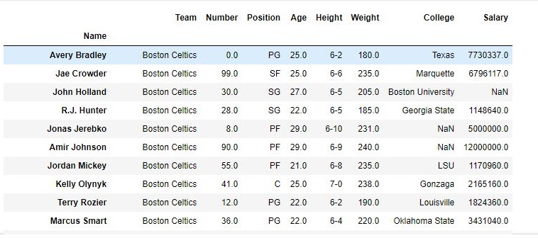
In his code, A list of index labels is passed and the rows corresponding to those labels are dropped using .drop() method.
# importing pandas module import pandas as pd # making data frame from csv file data = pd.read_csv("nba.csv", index_col ="Name" ) # dropping passed values data.drop(["Avery Bradley", "John Holland", "R.J. Hunter", "R.J. Hunter"], inplace = True) # display data |
Output:
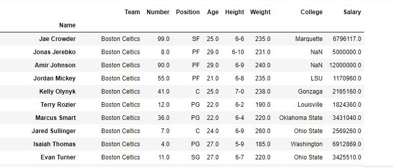
As shown in the output images, the new output doesn’t have the passed values. Those values were dropped and the changes were made in the original data frame since inplace was True.
Data Frame before Dropping values-
Data Frame after Dropping values-
Example #2 : Dropping columns with column name
In his code, Passed columns are dropped using column names. axis parameter is kept 1 since 1 refers to columns.
# importing pandas module import pandas as pd # making data frame from csv file data = pd.read_csv("nba.csv", index_col ="Name" ) # dropping passed columns data.drop(["Team", "Weight"], axis = 1, inplace = True) # display data |
Output:
As shown in the output images, the new output doesn’t have the passed columns. Those values were dropped since axis was set equal to 1 and the changes were made in the original data frame since inplace was True.
Data Frame before Dropping Columns-
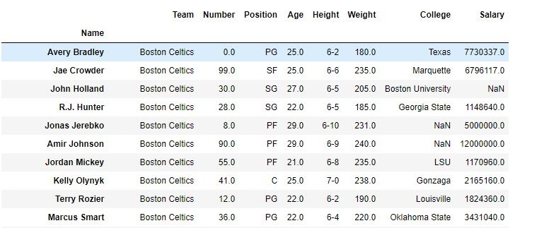
Data Frame after Dropping Columns-
###############################DATA FRAMES #####################
import pandas as pd
import numpy as np
df=pd.DataFrame()
print(df)
# List
l=[1,2,3,4]
df=pd.DataFrame(l,columns=['age'],index=["one","two","three","four"])
print(df)
# List of lists
df=pd.DataFrame([['a',21],['b',20],['c',22]],columns=["name",'age'],index=["one","two","three"])
print(df)
# Dictionary
df=pd.DataFrame({'name':['a','b','c'],'age':[21,20,22]},index=["one","two","three"])
print(df)
# List of dictionaries
df=pd.DataFrame([{'a':21,'b':20,'c':22},{'a':19,'b':18,'c':17}],index=["one","two"])
print(df)
# Select Column
print(df['a'])
# Column Addition
print(df['a']+df['b'])
#Append new column
df['d']=df['a']+df['b']
print(df)
# Delete column
del df['d']
print(df)
# Select row
print(df.loc['one'])
# row Addition
#print(df['one']+df['two'])
# Delete column
df=df.drop('one')
print(df)
################assignment#############################
import pandas as pd
import numpy as np
labels= ['name','roll_no','s1','s2','s3','s4']
#df=pd.DataFrame([{"x1",123,50,60,65,70],["x2",124,53,24,65,80],["x3",125,57,70,45,90]]}
#print(df)
df=pd.DataFrame([{'name':'x1','roll_no':123,'s1':50,'s2':50,'s3':50},
{'name':'x2','roll_no':124,'s1':55,'s2':57,'s3':56},])
#df=pd.DataFrame[d,columns=('name','roll_no','s1','s2','s3','s4')]
#df.columns = [labels]
print(df)
print(df['s1'])
print(df['s2'])
print(df['s1']+df["s2"])
df['total']=df['s1']+df['s2']+df['s3']
print(df)
df['avg']=df['total']/3
print(df)
bins=[0,50,60,70,80,90,100]
grade=['F','E','D','C','B','A']
df['Grade']=pd.cut(df['avg'],bins, labels=grade)
#df['grade']=df['avg']
print(df)
#########################
##################################
import os
import pandas as pd
#1: Import the excel file and call it xls_file
excel_file = pd.ExcelFile('enquiries.xls')
#2. View the excel_file's sheet names
print(excel_file.sheet_names)
#3 : Read an excel file using read_excel() method of pandas.
# read by default 1st sheet of an excel file
dataframe1 = pd.read_excel('enquiries.xls')
print(dataframe1)
#4. read 2nd sheet of an excel file replace missing values with nan
# By default Python treats blank values as NAN
# To treat any other garbage values like '??', "?????" we need to instruct using paramaetr na_values
#dataframe2 = pd.read_excel('enquiries.xls', sheet_name = 1,na_values=["??","????"])
# Type casting a column
5. dataframe2 ["Name]"= dataframe2 ["Name]".astype("object")
# total bytes by the column
5. dataframe2 ["Name]"= dataframe2 ["Name]".nbytes
# Replace One word with value under col 'Name'
5. dataframe2 ["Name]".replace('one',1,inplace=true)
# total no of null values in a data frame
5. dataframe2.isnull.sum()
#7 Access each value in a column using loop
l=df['age']
print(len(l))
for i in range(len(l)):
print(df['age'][i])
#8 append new column and find each age is adult or not
df.insert(2,"adult","")
# Access each value in a column using loop and
l=df['age']
print(len(l))
for i in range(len(l)):
print(df['age'][i])
if (df['age'][i] < 20):
df['adult'][i] ='yes'
else:
df['adult'][i] ='no'
# Find all values under column age
l=df['age'].get_values()
print(l)
# Find total unique values under column age
l=df['age'].value_counts()
print(l)
# Function on col to create new col uwith updated values i.e ages using function
#Create new column
df.insert(2,"new age","")
def incr_age(v):
return v+2
df['new age']=incr_age(df['age'])
print(df)
#4. read 2nd sheet of an excel file
#dataframe2 = pd.read_excel('enquiries.xls', sheet_name = 1,)
#5 : Read an excel file using read_excel() method of pandas.
db=pd.read_excel("enquiries.xls",sheet_name="Python")
#print(db)
#6: Load the excel_file's Sheet1 as a dataframe
df = excel_file.parse('Python')
print(df)
require_cols = [2]
#7. only read specific columns from an excel file
required_df = pd.read_excel('enquiries.xls', usecols = require_cols)
print(required_df)
#8 Handling missing data using 'na_values' parameter of the read_excel() method.
dataframe = pd.read_excel('enquiries.xls', na_values = "Missing",
sheet_name = "Python")
print(dataframe)
#9 : Skip starting rows when Reading an Excel File using 'skiprows' parameter of read_excel() method.
df = pd.read_excel('enquiries.xls', sheet_name = "Python", skiprows = 2)
print(df)
#10 #6 : Set the header to any row and start reading from that row, using 'header' parameter of the read_excel() method.
# setting the 3rd row as header.
df = pd.read_excel('enquiries.xls', sheet_name = "Python", header = 2)
print(df)
#11 : Reading Multiple Excel Sheets using 'sheet_name' parameter of the read_excel()method.
# read both 1st and 2nd sheet.
df = pd.read_excel('enquiries.xls', na_values = "Mssing", sheet_name =[0, 1])
print(df)
#12 Reading all Sheets of the excel file together using 'sheet_name' parameter of the read_excel() method.
# read all sheets together.
all_sheets_df = pd.read_excel('enquiries.xls', na_values = "Missing",
sheet_name = None)
print(all_sheets_df)
#13 retrieving columns by indexing operator
df = pd.read_excel('enquiries.xls', na_values = "Mssing", sheet_name ="Python")
print(df)
first = df["Mob Num"]
print(first)
# 14 Shallow caopy
df2=df
print(df2)
df3=df.copy(deep=False)
print(df3)
# 15 Deep copy
df3=df.copy(deep=True)
print(df3)
#16 Get Row labels
print(df3.index)
#17 Get columns labels
print(df3.columns)
#18 Get columns labels
print(df3.size)
#19 Get columns labels
print(df3.shape)
#20 Get memory usage
print(df3.memory_usage)
#21 Get first 5 rows
print(df3.head(5))
#22 Get lst 5 rows
print(df3.tail(5))
#23 Indexing row=integer and column=label name
#Arshia.Shaik
#Value at row 4 and column "Name"
print(df3.at[4,"Name"])
#23 Indexing row=integer and column=label name
#Arshia.Shaik
#Value at row 4 and column "Name"
print(df3.iat[4,1])
#24 Indexing group of rows and columns
#all rows with only column="Name"
#Arshia.Shaik
#Value at row 4 and column "Name"
print(df3.loc[:,"Name"])
print(df3.loc[[900,901],["Name","E.mail"]])
################### MISSING VALUES########################
# Dictionary
df=pd.DataFrame({'name':['a','b','a'],'age':[21,20,32]},index=["one","two","three"])
print(df)
# Is there any nan(not a number) values i.e blank
# returns data frame of boolean values
print(df.isna())
## Is there any nan values i.e blank
print(df.isnull())
# count the total nan values against eash column
print(df.isna().sum())
#count the total nan values against eash column
print(df.isnull().sum())
#Sub setting the rows that have one or more missing values
missing=df[df.isnull().any(axis=1)]
# Statistical details about the frame
# for each col, mean, median, etc
print(df.describe())
# To get mean of column
print(df['age'].mean())
# To fill missing value with mean in the col 'age'
#fillna() fills the missed values
df['age'].fillna(df['age'].mean(),inplace=True)
# returns a series labelled 1d array
# How many times each unique value is repated
print(df['name'].value_counts())
# To access first item in the series
print(df['name'].value_counts().index[0])
df['name'].fillna(df['name'].value_counts().index[0],inplace=True)
######
################################################
# Dictionary
df=pd.DataFrame({'name':['a','b','c'],'age':[21,20,22]},index=["one","two","three"])
print(df)
# return the dtype of each column
print( df.dtypes)
# return the no of columns for each dtype
print( df.dtypes.value_counts())
# return the no of rows including only object type cols
print( df.select_dtypes(include=[object]))
# return the no of rows excluding only object type cols
print( df.select_dtypes(exclude=[object]))
# return the no of rows excluding only object type cols
# no of cols , rows and memory usage
print( df.info())
# return the unique elementys of the col values
# np.unique(array)
print( np.unique(df['name']))
################################3