
Decision Tree
Decision Tree : Decision tree is the most powerful and popular tool for classification and prediction. A Decision tree is a flowchart like tree structure, where each internal node denotes a test on an attribute, each branch represents an outcome of the test, and each leaf node (terminal node) holds a class label.
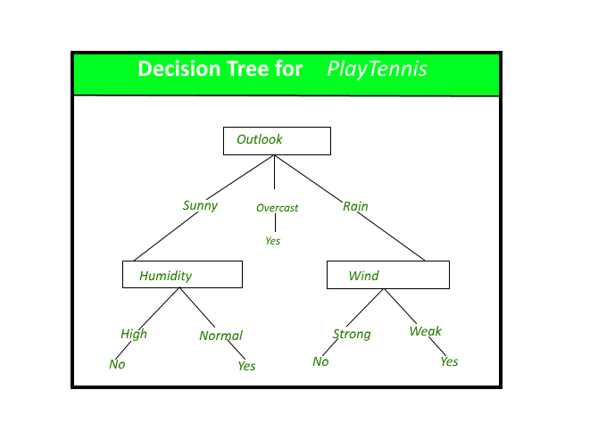
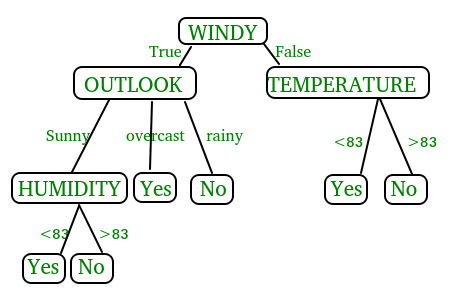
A decision tree for the concept PlayTennis.
Construction of Decision Tree :
A tree can be “learned” by splitting the source set into subsets based on an attribute value test. This process is repeated on each derived subset in a recursive manner called recursive partitioning. The recursion is completed when the subset at a node all has the same value of the target variable, or when splitting no longer adds value to the predictions. The construction of decision tree classifier does not require any domain knowledge or parameter setting, and therefore is appropriate for exploratory knowledge discovery. Decision trees can handle high dimensional data. In general decision tree classifier has good accuracy. Decision tree induction is a typical inductive approach to learn knowledge on classification.
Decision Tree Representation :
Decision trees classify instances by sorting them down the tree from the root to some leaf node, which provides the classification of the instance. An instance is classified by starting at the root node of the tree,testing the attribute specified by this node,then moving down the tree branch corresponding to the value of the attribute as shown in the above figure.This process is then repeated for the subtree rooted at the new node.
The decision tree in above figure classifies a particular morning according to whether it is suitable for playing tennis and returning the classification associated with the particular leaf.(in this case Yes or No).
For example,the instance
(Outlook = Rain, Temperature = Hot, Humidity = High, Wind = Strong )
would be sorted down the leftmost branch of this decision tree and would therefore be classified as a negative instance.
In other words we can say that decision tree represent a disjunction of conjunctions of constraints on the attribute values of instances.
(Outlook = Sunny ^ Humidity = Normal) v (Outllok = Overcast) v (Outlook = Rain ^ Wind = Weak)
Strengths and Weakness of Decision Tree approach
The strengths of decision tree methods are:
- Decision trees are able to generate understandable rules.
- Decision trees perform classification without requiring much computation.
- Decision trees are able to handle both continuous and categorical variables.
- Decision trees provide a clear indication of which fields are most important for prediction or classification.
The weaknesses of decision tree methods :
- Decision trees are less appropriate for estimation tasks where the goal is to predict the value of a continuous attribute.
- Decision trees are prone to errors in classification problems with many class and relatively small number of training examples.
- Decision tree can be computationally expensive to train. The process of growing a decision tree is computationally expensive. At each node, each candidate splitting field must be sorted before its best split can be found. In some algorithms, combinations of fields are used and a search must be made for optimal combining weights. Pruning algorithms can also be expensive since many candidate sub-trees must be formed and compared.
Decision Tree Introduction with example
- Decision tree algorithm falls under the category of supervised learning. They can be used to solve both regression and classification problems.
- Decision tree uses the tree representation to solve the problem in which each leaf node corresponds to a class label and attributes are represented on the internal node of the tree.
- We can represent any boolean function on discrete attributes using the decision tree.
Below are some assumptions that we made while using decision tree:
- At the beginning, we consider the whole training set as the root.
- Feature values are preferred to be categorical. If the values are continuous then they are discretized prior to building the model.
- On the basis of attribute values records are distributed recursively.
- We use statistical methods for ordering attributes as root or the internal node.
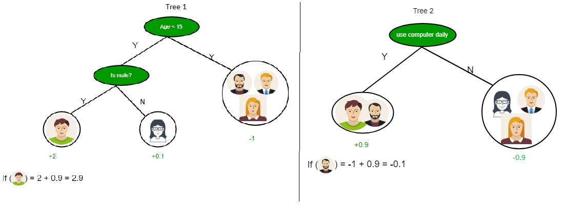
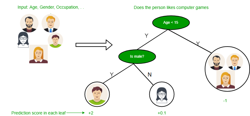
As you can see from the above image that Decision Tree works on the Sum of Product form which is also known as Disjunctive Normal Form. In the above image, we are predicting the use of computer in the daily life of the people.
In Decision Tree the major challenge is to identification of the attribute for the root node in each level. This process is known as attribute selection. We have two popular attribute selection measures:
- Information Gain
- Gini Index
1. Information Gain
When we use a node in a decision tree to partition the training instances into smaller subsets the entropy changes. Information gain is a measure of this change in entropy.
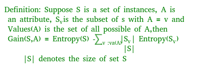
Definition: Suppose S is a set of instances, A is an attribute, Sv is the subset of S with A = v, and Values (A) is the set of all possible values of A, then

Entropy
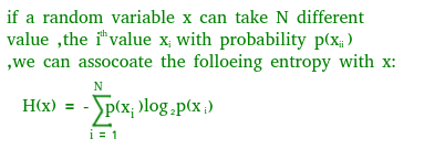
Entropy is the measure of uncertainty of a random variable, it characterizes the impurity of an arbitrary collection of examples. The higher the entropy more the information content.
Definition: Suppose S is a set of instances, A is an attribute, Sv is the subset of S with A = v, and Values (A) is the set of all possible values of A, then
Example:
For the set X = {a,a,a,b,b,b,b,b}
Total intances: 8
Instances of b: 5
Instances of a: 3
![Entropy H(X) = -\left [ \left ( \frac{3}{8} \right )log_{2}\frac{3}{8} + \left ( \frac{5}{8} \right )log_{2}\frac{5}{8} \right ]](https://www.geeksforgeeks.org/wp-content/ql-cache/quicklatex.com-4b2ec6c432a20a955f66ed0da0c5ad3e_l3.svg "Rendered by QuickLaTeX.com") = -[0.375 * (-1.415) + 0.625 * (-0.678)]
=-(-0.53-0.424)
= 0.954
= -[0.375 * (-1.415) + 0.625 * (-0.678)]
=-(-0.53-0.424)
= 0.954
Building Decision Tree using Information Gain
The essentials:
-
- Start with all training instances associated with the root node
- Use info gain to choose which attribute to label each node with
- Note: No root-to-leaf path should contain the same discrete attribute twice
- Recursively construct each subtree on the subset of training instances that would be classified down that path in the tree.
The border cases:
- If all positive or all negative training instances remain, label that node “yes” or “no” accordingly
- If no attributes remain, label with a majority vote of training instances left at that node
- If no instances remain, label with a majority vote of the parent’s training instances
Example:
Now, lets draw a Decision Tree for the following data using Information gain.
Training set: 3 features and 2 classes
| X | Y | Z | C |
|---|---|---|---|
| 1 | 1 | 1 | I |
| 1 | 1 | 0 | I |
| 0 | 0 | 1 | II |
| 1 | 0 | 0 | II |
Here, we have 3 features and 2 output classes.
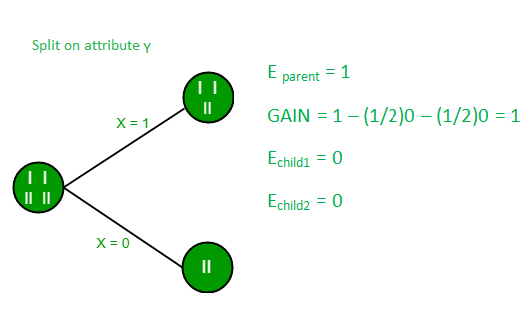
To build a decision tree using Information gain. We will take each of the feature and calculate the information for each feature.
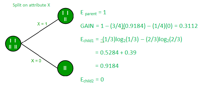
Split on feature X
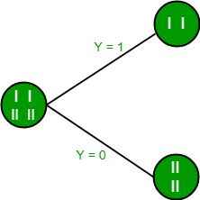
Split on feature Y
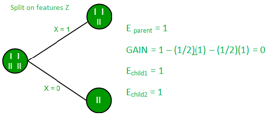
Split on feature Z
From the above images we can see that the information gain is maximum when we make a split on feature Y. So, for the root node best suited feature is feature Y. Now we can see that while splitting the dataset by feature Y, the child contains pure subset of the target variable. So we don’t need to further split the dataset.
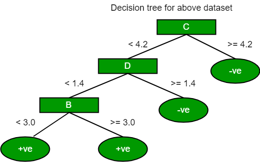
The final tree for the above dataset would be look like this:
2. Gini Index
-
- Gini Index is a metric to measure how often a randomly chosen element would be incorrectly identified.
- It means an attribute with lower Gini index should be preferred.
- Sklearn supports “Gini” criteria for Gini Index and by default, it takes “gini” value.
- The Formula for the calculation of the of the Gini Index is given below.

Example:
Lets consider the dataset in the image below and draw a decision tree using gini index.
| INDEX | A | B | C | D | E |
|---|---|---|---|---|---|
| 1 | 4.8 | 3.4 | 1.9 | 0.2 | positive |
| 2 | 5 | 3 | 1.6 | 1.2 | positive |
| 3 | 5 | 3.4 | 1.6 | 0.2 | positive |
| 4 | 5.2 | 3.5 | 1.5 | 0.2 | positive |
| 5 | 5.2 | 3.4 | 1.4 | 0.2 | positive |
| 6 | 4.7 | 3.2 | 1.6 | 0.2 | positive |
| 7 | 4.8 | 3.1 | 1.6 | 0.2 | positive |
| 8 | 5.4 | 3.4 | 1.5 | 0.4 | positive |
| 9 | 7 | 3.2 | 4.7 | 1.4 | negative |
| 10 | 6.4 | 3.2 | 4.7 | 1.5 | negative |
| 11 | 6.9 | 3.1 | 4.9 | 1.5 | negative |
| 12 | 5.5 | 2.3 | 4 | 1.3 | negative |
| 13 | 6.5 | 2.8 | 4.6 | 1.5 | negative |
| 14 | 5.7 | 2.8 | 4.5 | 1.3 | negative |
| 15 | 6.3 | 3.3 | 4.7 | 1.6 | negative |
| 16 | 4.9 | 2.4 | 3.3 | 1 | negative |
In the dataset above there are 5 attributes from which attribute E is the predicting feature which contains 2(Positive & Negative) classes. We have an equal proportion for both the classes.
In Gini Index, we have to choose some random values to categorize each attribute. These values for this dataset are:
    A       B        C         D
  >= 5     >= 3.0      >= 4.2    >= 1.4
   < 5      < 3.0       < 4.2     < 1.4
Calculating Gini Index for Var A:
Value >= 5: 12
Attribute A >= 5 & class = positive: 
Attribute A >= 5 & class = negative: 
Gini(5, 7) = 1 – ![\left [ \left ( \frac{5}{12} \right )^{2} + \left ( \frac{7}{12} \right )^{2}\right ] = 0.4860](https://www.geeksforgeeks.org/wp-content/ql-cache/quicklatex.com-9e4da24121695bf83629d453d625b97a_l3.svg "Rendered by QuickLaTeX.com")
Value < 5: 4
Attribute A < 5 & class = positive: 
Attribute A < 5 & class = negative: 
Gini(3, 1) = 1 – ![\left [ \left ( \frac{3}{4} \right )^{2} + \left ( \frac{1}{4} \right )^{2}\right ] = 0.375](https://www.geeksforgeeks.org/wp-content/ql-cache/quicklatex.com-cd839511a4c9b5d7a8253d8b21cb5e5a_l3.svg "Rendered by QuickLaTeX.com")
By adding weight and sum each of the gini indices:

Calculating Gini Index for Var B:
Value >= 3: 12
Attribute B >= 3 & class = positive: 
Attribute B >= 5 & class = negative: 
Gini(5, 7) = 1 – ![\left [ \left ( \frac{8}{12} \right )^{2} + \left ( \frac{4}{12} \right )^{2}\right ] = 0.4460](https://www.geeksforgeeks.org/wp-content/ql-cache/quicklatex.com-e51ae059395978963276fb4824fdd76e_l3.svg "Rendered by QuickLaTeX.com")
Value < 3: 4
Attribute A < 3 & class = positive: 
Attribute A < 3 & class = negative: 
Gini(3, 1) = 1 – ![\left [ \left ( \frac{0}{4} \right )^{2} + \left ( \frac{4}{4} \right )^{2}\right ] = 1](https://www.geeksforgeeks.org/wp-content/ql-cache/quicklatex.com-f9a8e3f184b7cbcf5ff48ae37a627a98_l3.svg "Rendered by QuickLaTeX.com")
By adding weight and sum each of the gini indices:

Using the same approach we can calculate the Gini index for C and D attributes.
             Positive    Negative
For A|>= 5.0    5       7
     |<5    3       1
Ginin Index of A = 0.45825
             Positive    Negative
For B|>= 3.0    8       4
     |< 3.0    0       4
Gini Index of B= 0.3345
             Positive    Negative
For C|>= 4.2    0       6
     |< 4.2    8       2
Gini Index of C= 0.2
             Positive    Negative
For D|>= 1.4    0       5
     |< 1.4    8       3
Gini Index of D= 0.273
The most notable types of decision tree algorithms are:-
1. Iterative Dichotomiser 3 (ID3): This algorithm uses Information Gain to decide which attribute is to be used classify the current subset of the data. For each level of the tree, information gain is calculated for the remaining data recursively.
2. C4.5: This algorithm is the successor of the ID3 algorithm. This algorithm uses either Information gain or Gain ratio to decide upon the classifying attribute. It is a direct improvement from the ID3 algorithm as it can handle both continuous and missing attribute values.
3. Classification and Regression Tree(CART): It is a dynamic learning algorithm which can produce a regression tree as well as a classification tree depending upon the dependent variable.
Reference: dataaspirant
Decision tree implementation using Python
Prerequisites: Decision Tree, DecisionTreeClassifier, sklearn, numpy, pandas
Decision Tree is one of the most powerful and popular algorithm. Decision-tree algorithm falls under the category of supervised learning algorithms. It works for both continuous as well as categorical output variables.
In this article, We are going to implement a Decision tree algorithm on the Balance Scale Weight & Distance Database presented on the UCI.
Data-set Description :
Title          : Balance Scale Weight & Distance Database
Number of Instances: 625 (49 balanced, 288 left, 288 right)
Number of Attributes: 4 (numeric) + class name = 5
Attribute Information:
-
- Class Name (Target variable): 3
- L [balance scale tip to the left]
- B [balance scale be balanced]
- R [balance scale tip to the right]
- Left-Weight: 5 (1, 2, 3, 4, 5)
- Left-Distance: 5 (1, 2, 3, 4, 5)
- Right-Weight: 5 (1, 2, 3, 4, 5)
- Right-Distance: 5 (1, 2, 3, 4, 5)
- Class Name (Target variable): 3
Missing Attribute Values
-
- : None
Class Distribution:
-
-
- 46.08 percent are L
- 07.84 percent are B
- 46.08 percent are R
You can find more details of the dataset
-
- .
Used Python Packages :
- sklearn :
- In python, sklearn is a machine learning package which include a lot of ML algorithms.
- Here, we are using some of its modules like train_test_split, DecisionTreeClassifier and accuracy_score.
- NumPy :
- It is a numeric python module which provides fast maths functions for calculations.
- It is used to read data in numpy arrays and for manipulation purpose.
- Pandas :
- Used to read and write different files.
- Data manipulation can be done easily with dataframes.
Installation of the packages :
In Python, sklearn is the package which contains all the required packages to implement Machine learning algorithm. You can install the sklearn package by following the commands given below.
using pip :
pip install -U scikit-learn
Before using the above command make sure you have scipy and numpy packages installed.
If you don’t have pip. You can install it using
python get-pip.py
using conda :
conda install scikit-learn
Assumptions we make while using Decision tree :
-
- At the beginning, we consider the whole training set as the root.
- Attributes are assumed to be categorical for information gain and for gini index, attributes are assumed to be continuous.
- On the basis of attribute values records are distributed recursively.
- We use statistical methods for ordering attributes as root or internal node.
Pseudocode :
-
-
- Find the best attribute and place it on the root node of the tree.
- Now, split the training set of the dataset into subsets. While making the subset make sure that each subset of training dataset should have the same value for an attribute.
- Find leaf nodes in all branches by repeating 1 and 2 on each subset.
-
While implementing the decision tree we will go through the following two phases:
-
-
- Building Phase
- Preprocess the dataset.
- Split the dataset from train and test using Python sklearn package.
- Train the classifier.
- Operational Phase
- Make predictions.
- Calculate the accuracy.
- Building Phase
-
Data Import :
-
- To import and manipulate the data we are using the pandas package provided in python.
- Here, we are using a URL which is directly fetching the dataset from the UCI site no need to download the dataset. When you try to run this code on your system make sure the system should have an active Internet connection.
- As the dataset is separated by “,” so we have to pass the sep parameter’s value as “,”.
- Another thing is notice is that the dataset doesn’t contain the header so we will pass the Header parameter’s value as none. If we will not pass the header parameter then it will consider the first line of the dataset as the header.
Data Slicing :
-
- Before training the model we have to split the dataset into the training and testing dataset.
- To split the dataset for training and testing we are using the sklearn module train_test_split
- First of all we have to separate the target variable from the attributes in the dataset.
X = balance_data.values[:, 1:5]
Y = balance_data.values[:,0]
-
- Above are the lines from the code which separate the dataset. The variable X contains the attributes while the variable Y contains the target variable of the dataset.
- Next step is to split the dataset for training and testing purpose.
X_train, X_test, y_train, y_test = train_test_split(
          X, Y, test_size = 0.3, random_state = 100)
-
- Above line split the dataset for training and testing. As we are splitting the dataset in a ratio of 70:30 between training and testing so we are pass test_size parameter’s value as 0.3.
- random_state variable is a pseudo-random number generator state used for random sampling.
Terms used in code :
Gini index and information gain both of these methods are used to select from the n attributes of the dataset which attribute would be placed at the root node or the internal node.
Gini index
![]()
-
- Gini Index is a metric to measure how often a randomly chosen element would be incorrectly identified.
- It means an attribute with lower gini index should be preferred.
- Sklearn supports “gini” criteria for Gini Index and by default, it takes “gini” value.
Entropy
-
- Entropy is the measure of uncertainty of a random variable, it characterizes the impurity of an arbitrary collection of examples. The higher the entropy the more the information content.
Information Gain
-
- The entropy typically changes when we use a node in a decision tree to partition the training instances into smaller subsets. Information gain is a measure of this change in entropy.
- Sklearn supports “entropy” criteria for Information Gain and if we want to use Information Gain method in sklearn then we have to mention it explicitly.
Accuracy score
-
- Accuracy score is used to calculate the accuracy of the trained classifier.
Confusion Matrix
-
- Confusion Matrix is used to understand the trained classifier behavior over the test dataset or validate dataset.
Below is the python code for the decision tree.
# Run this program on your local python # interpreter, provided you have installed # the required libraries. # Importing the required packages import numpy as np import pandas as pd from sklearn.metrics import confusion_matrix from sklearn.cross_validation import train_test_split from sklearn.tree import DecisionTreeClassifier from sklearn.metrics import accuracy_score from sklearn.metrics import classification_report # Function importing Dataset def importdata(): balance_data = pd.read_csv( 'databases/balance-scale/balance-scale.data', sep= ',', header = None) # Printing the dataswet shape print ("Dataset Length: ", len(balance_data)) print ("Dataset Shape: ", balance_data.shape) # Printing the dataset obseravtions print ("Dataset: ",balance_data.head()) return balance_data # Function to split the dataset def splitdataset(balance_data): # Separating the target variable X = balance_data.values[:, 1:5] Y = balance_data.values[:, 0] # Splitting the dataset into train and test X_train, X_test, y_train, y_test = train_test_split( X, Y, test_size = 0.3, random_state = 100) return X, Y, X_train, X_test, y_train, y_test # Function to perform training with giniIndex. def train_using_gini(X_train, X_test, y_train): # Creating the classifier object clf_gini = DecisionTreeClassifier(criterion = "gini", random_state = 100,max_depth=3, min_samples_leaf=5) # Performing training clf_gini.fit(X_train, y_train) return clf_gini # Function to perform training with entropy. def tarin_using_entropy(X_train, X_test, y_train): # Decision tree with entropy clf_entropy = DecisionTreeClassifier( criterion = "entropy", random_state = 100, max_depth = 3, min_samples_leaf = 5) # Performing training clf_entropy.fit(X_train, y_train) return clf_entropy # Function to make predictions def prediction(X_test, clf_object): # Predicton on test with giniIndex y_pred = clf_object.predict(X_test) print("Predicted values:") print(y_pred) return y_pred # Function to calculate accuracy def cal_accuracy(y_test, y_pred): print("Confusion Matrix: ", confusion_matrix(y_test, y_pred)) print ("Accuracy : ", accuracy_score(y_test,y_pred)*100) print("Report : ", classification_report(y_test, y_pred)) # Driver code def main(): # Building Phase data = importdata() X, Y, X_train, X_test, y_train, y_test = splitdataset(data) clf_gini = train_using_gini(X_train, X_test, y_train) clf_entropy = tarin_using_entropy(X_train, X_test, y_train) # Operational Phase print("Results Using Gini Index:") # Prediction using gini y_pred_gini = prediction(X_test, clf_gini) cal_accuracy(y_test, y_pred_gini) print("Results Using Entropy:") # Prediction using entropy y_pred_entropy = prediction(X_test, clf_entropy) cal_accuracy(y_test, y_pred_entropy) # Calling main function if __name__=="__main__": main() |
Data Infomation:
Dataset Length:  625
Dataset Shape:  (625, 5)
Dataset:     0  1  2  3  4
0  B  1  1  1  1
1  R  1  1  1  2
2  R  1  1  1  3
3  R  1  1  1  4
4  R  1  1  1  5
Results Using Gini Index:
Predicted values:
['R' 'L' 'R' 'R' 'R' 'L' 'R' 'L' 'L' 'L' 'R' 'L' 'L' 'L' 'R' 'L' 'R' 'L'
 'L' 'R' 'L' 'R' 'L' 'L' 'R' 'L' 'L' 'L' 'R' 'L' 'L' 'L' 'R' 'L' 'L' 'L'
 'L' 'R' 'L' 'L' 'R' 'L' 'R' 'L' 'R' 'R' 'L' 'L' 'R' 'L' 'R' 'R' 'L' 'R'
 'R' 'L' 'R' 'R' 'L' 'L' 'R' 'R' 'L' 'L' 'L' 'L' 'L' 'R' 'R' 'L' 'L' 'R'
 'R' 'L' 'R' 'L' 'R' 'R' 'R' 'L' 'R' 'L' 'L' 'L' 'L' 'R' 'R' 'L' 'R' 'L'
 'R' 'R' 'L' 'L' 'L' 'R' 'R' 'L' 'L' 'L' 'R' 'L' 'R' 'R' 'R' 'R' 'R' 'R'
 'R' 'L' 'R' 'L' 'R' 'R' 'L' 'R' 'R' 'R' 'R' 'R' 'L' 'R' 'L' 'L' 'L' 'L'
 'L' 'L' 'L' 'R' 'R' 'R' 'R' 'L' 'R' 'R' 'R' 'L' 'L' 'R' 'L' 'R' 'L' 'R'
 'L' 'L' 'R' 'L' 'L' 'R' 'L' 'R' 'L' 'R' 'R' 'R' 'L' 'R' 'R' 'R' 'R' 'R'
 'L' 'L' 'R' 'R' 'R' 'R' 'L' 'R' 'R' 'R' 'L' 'R' 'L' 'L' 'L' 'L' 'R' 'R'
 'L' 'R' 'R' 'L' 'L' 'R' 'R' 'R']

Confusion Matrix:  [[ 0  6  7]
                    [ 0 67 18]
                    [ 0 19 71]]
Accuracy :  73.4042553191
Report :
       precision    recall  f1-score   support
  B       0.00      0.00      0.00        13
  L       0.73      0.79      0.76        85
  R       0.74      0.79      0.76        90
avg/total 0.68      0.73      0.71       188
Results Using Entropy:
Predicted values:
['R' 'L' 'R' 'L' 'R' 'L' 'R' 'L' 'R' 'R' 'R' 'R' 'L' 'L' 'R' 'L' 'R' 'L'
 'L' 'R' 'L' 'R' 'L' 'L' 'R' 'L' 'R' 'L' 'R' 'L' 'R' 'L' 'R' 'L' 'L' 'L'
 'L' 'L' 'R' 'L' 'R' 'L' 'R' 'L' 'R' 'R' 'L' 'L' 'R' 'L' 'L' 'R' 'L' 'L'
 'R' 'L' 'R' 'R' 'L' 'R' 'R' 'R' 'L' 'L' 'R' 'L' 'L' 'R' 'L' 'L' 'L' 'R'
 'R' 'L' 'R' 'L' 'R' 'R' 'R' 'L' 'R' 'L' 'L' 'L' 'L' 'R' 'R' 'L' 'R' 'L'
 'R' 'R' 'L' 'L' 'L' 'R' 'R' 'L' 'L' 'L' 'R' 'L' 'L' 'R' 'R' 'R' 'R' 'R'
 'R' 'L' 'R' 'L' 'R' 'R' 'L' 'R' 'R' 'L' 'R' 'R' 'L' 'R' 'R' 'R' 'L' 'L'
 'L' 'L' 'L' 'R' 'R' 'R' 'R' 'L' 'R' 'R' 'R' 'L' 'L' 'R' 'L' 'R' 'L' 'R'
 'L' 'R' 'R' 'L' 'L' 'R' 'L' 'R' 'R' 'R' 'R' 'R' 'L' 'R' 'R' 'R' 'R' 'R'
 'R' 'L' 'R' 'L' 'R' 'R' 'L' 'R' 'L' 'R' 'L' 'R' 'L' 'L' 'L' 'L' 'L' 'R'
 'R' 'R' 'L' 'L' 'L' 'R' 'R' 'R']

Confusion Matrix:  [[ 0  6  7]
                    [ 0 63 22]
                    [ 0 20 70]]
Accuracy :  70.7446808511
Report :
          precision    recall  f1-score   support
    B       0.00      0.00      0.00        13
    L       0.71      0.74      0.72        85
    R       0.71      0.78      0.74        90
avg / total 0.66      0.71      0.68       188
Python | Decision Tree Regression using sklearn
Decision Tree is a decision-making tool that uses a flowchart-like tree structure or is a model of decisions and all of their possible results, including outcomes, input costs and utility.
Decision-tree algorithm falls under the category of supervised learning algorithms. It works for both continuous as well as categorical output variables.
The branches/edges represent the result of the node and the nodes have either:
- Conditions [Decision Nodes]
- Result [End Nodes]
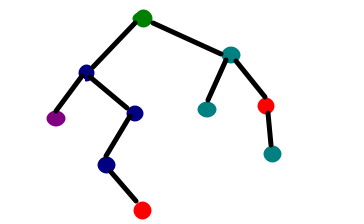
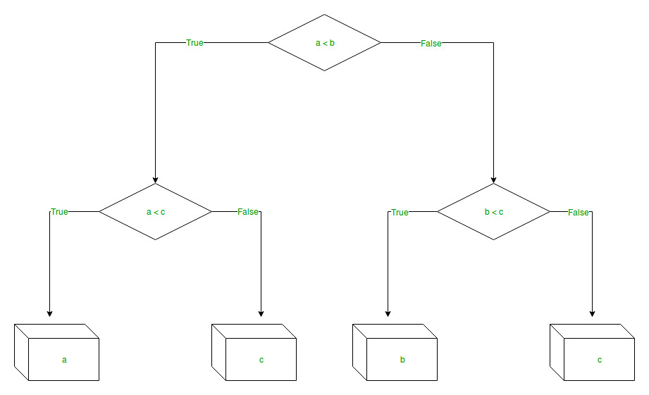
The branches/edges represent the truth/falsity of the statement and takes makes a decision based on that in the example below which shows a decision tree that evaluates the smallest of three numbers:
Decision Tree Regression:
Decision tree regression observes features of an object and trains a model in the structure of a tree to predict data in the future to produce meaningful continuous output. Continuous output means that the output/result is not discrete, i.e., it is not represented just by a discrete, known set of numbers or values.
Discrete output example: A weather prediction model that predicts whether or not there’ll be rain in a particular day.
Continuous output example: A profit prediction model that states the probable profit that can be generated from the sale of a product.
Here, continuous values are predicted with the help of a decision tree regression model.
Let’s see the Step-by-Step implementation –
- Step 1: Import the required libraries.
# import numpy package for arrays and stuffimportnumpy as np# import matplotlib.pyplot for plotting our resultimportmatplotlib.pyplot as plt# import pandas for importing csv filesimportpandas as pd - Step 2: Initialize and print the Dataset.
# import dataset# dataset = pd.read_csv('Data.csv')# alternatively open up .csv file to read datadataset=np.array([['Asset Flip',100,1000],['Text Based',500,3000],['Visual Novel',1500,5000],['2D Pixel Art',3500,8000],['2D Vector Art',5000,6500],['Strategy',6000,7000],['First Person Shooter',8000,15000],['Simulator',9500,20000],['Racing',12000,21000],['RPG',14000,25000],['Sandbox',15500,27000],['Open-World',16500,30000],['MMOFPS',25000,52000],['MMORPG',30000,80000]])# print the datasetprint(dataset)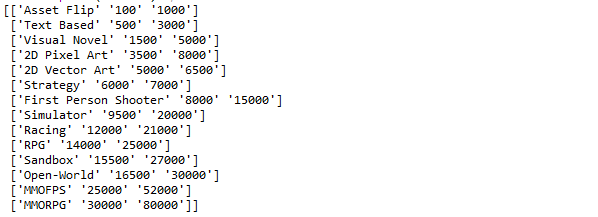
- Step 3: Select all the rows and column 1 from dataset to “X”.
# select all rows by : and column 1# by 1:2 representing featuresX=dataset[:,1:2].astype(int)# print Xprint(X)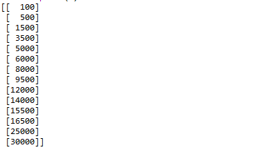
- Step 4: Select all of the rows and column 2 from dataset to “y”.
# select all rows by : and column 2# by 2 to Y representing labelsy=dataset[:,2].astype(int)# print yprint(y)
- Step 5: Fit decision tree regressor to the dataset
# import the regressorfromsklearn.treeimportDecisionTreeRegressor# create a regressor objectregressor=DecisionTreeRegressor(random_state=0)# fit the regressor with X and Y dataregressor.fit(X, y)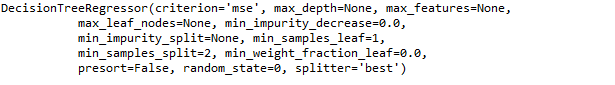
- Step 6: Predicting a new value
# predicting a new value# test the output by changing values, like 3750y_pred=regressor.predict(3750)# print the predicted priceprint("Predicted price: % d\n"%y_pred)
- Step 7: Visualising the result
# arange for creating a range of values# from min value of X to max value of X# with a difference of 0.01 between two# consecutive valuesX_grid=np.arange(min(X),max(X),0.01)# reshape for reshaping the data into# a len(X_grid)*1 array, i.e. to make# a column out of the X_grid valuesX_grid=X_grid.reshape((len(X_grid),1))# scatter plot for original dataplt.scatter(X, y, color='red')# plot predicted dataplt.plot(X_grid, regressor.predict(X_grid), color='blue')# specify titleplt.title('Profit to Production Cost (Decision Tree Regression)')# specify X axis labelplt.xlabel('Production Cost')# specify Y axis labelplt.ylabel('Profit')# show the plotplt.show()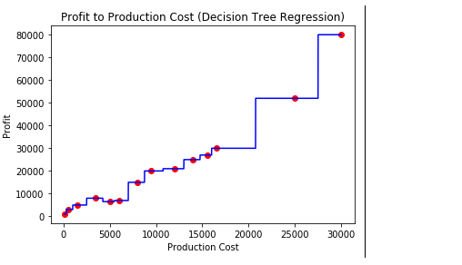
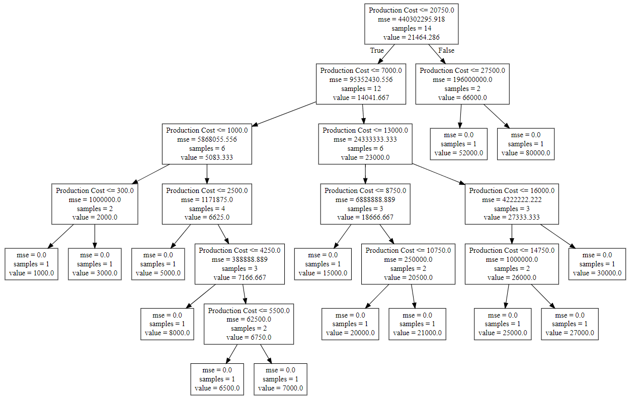
- Step 8: The tree is finally exported and shown in the TREE STRUCTURE below, visualized using http://www.webgraphviz.com/ by copying the data from the ‘tree.dot’ file.
# import export_graphvizfromsklearn.treeimportexport_graphviz# export the decision tree to a tree.dot file# for visualizing the plot easily anywhereexport_graphviz(regressor, out_file='tree.dot',feature_names=['Production Cost'])
Output (Decision Tree):
sklearn.Binarizer() in Python
sklearn.preprocessing.Binarizer() is a method which belongs to preprocessing module. It plays a key role in the discretization of continuous feature values.
Example #1:
A continuous data of pixels values of an 8-bit grayscale image have values ranging between 0 (black) and 255 (white) and one needs it to be black and white. So, using Binarizer() one can set a threshold converting pixel values from 0 – 127 to 0 and 128 – 255 as 1.
Example #2:
One has a machine record having “Success Percentage” as a feature. These values are continuous ranging from 10% to 99% but a researcher simply wants to use this data for prediction of pass or fail status for the machine based on other given parameters.
Syntax :
sklearn.preprocessing.Binarizer(threshold, copy)
Parameters :
threshold :[float, optional] Values less than or equal to threshold is mapped to 0, else to 1. By default threshold value is 0.0.
copy :[boolean, optional] If set to False, it avoids a copy. By default it is True.
Return :
Binarized Feature values
Download the dataset:
Go to the link and download Data.csv
Below is the Python code explaning sklearn.Binarizer()
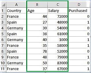
# Python code explaining how # to Binarize feature values """ PART 1 Importing Libraries """ import numpy as np import matplotlib.pyplot as plt import pandas as pd # Sklearn library from sklearn import preprocessing """ PART 2 Importing Data """ data_set = pd.read_csv( 'C:\\Users\\dell\\Desktop\\Data_for_Feature_Scaling.csv') data_set.head() # here Features - Age and Salary columns # are taken using slicing # to binarize values age = data_set.iloc[:, 1].values salary = data_set.iloc[:, 2].values print ("\nOriginal age data values : \n", age) print ("\nOriginal salary data values : \n", salary) """ PART 4 Binarizing values """ from sklearn.preprocessing import Binarizer x = age x = x.reshape(1, -1) y = salary y = y.reshape(1, -1) # For age, let threshold be 35 # For salary, let threshold be 61000 binarizer_1 = Binarizer(35) binarizer_2 = Binarizer(61000) # Transformed feature print ("\nBinarized age : \n", binarizer_1.fit_transform(x)) print ("\nBinarized salary : \n", binarizer_2.fit_transform(y)) |
Output :
   Country  Age  Salary  Purchased
0   France   44   72000          0
1    Spain   27   48000          1
2  Germany   30   54000          0
3    Spain   38   61000          0
4  Germany   40    1000          1

Original age data values :
 [44 27 30 38 40 35 78 48 50 37]

Original salary data values :
 [72000 48000 54000 61000  1000 58000 52000 79000 83000 67000]

Binarized age :
 [[1 0 0 1 1 0 1 1 1 1]]

Binarized salary :
 [[1 0 0 0 0 0 0 1 1 1]]