ML | Why Logistic Regression in Classification ?

Using Linear Regression, all predictions >= 0.5 can be considered as 1 and rest all < 0.5 can be considered as 0. But then the question arises why classification can’t be performed using it?

Problem –

Suppose we are classifying a mail as spam or not spam and our output is y, it can be 0(spam) or 1(not spam). In case of Linear Regression, h_θ(x) can be > 1 or < 0. Although our prediction should be in between 0 and 1, the model will predict value out of the range i.e. maybe > 1 or < 0.

So, that’s why for a Classification task, Logistic/Sigmoid Regression plays its role.

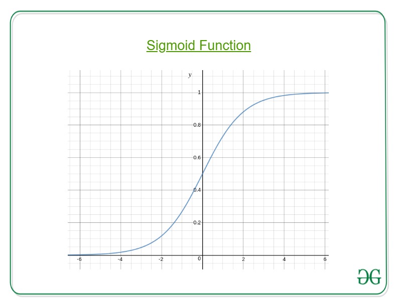
$h_{\Theta} (x) = g (\Theta ^{T}x) z = \Theta ^{T}x g(z) = \frac{1}{1+e^{-z}}$

Here, we plug θ^Tx into logistic function where θ are the weights/parameters and x is the input and h_θ(x) is the hypothesis function. g() is the sigmoid function.

$h_{\Theta} (x) = P( y =1 | x ; \Theta )$

It means that y = 1 probability when x is parameterized to θ

To get the discrete values 0 or 1 for classification, discrete boundaries are defined. The hypothesis function cab be translated as

$h_{\Theta} (x) \geq 0.5 \rightarrow y = 1 h_{\Theta} (x) < 0.5 \rightarrow y = 0$

${g(z) \geq 0.5} \\ {\Rightarrow \Theta ^{T}x \geq 0.5} \\ {\Rightarrow z \geq 0.5 }$

Decision Boundary is the line that distinguishes the area where y=0 and where y=1. These decision boundaries result from the hypothesis function under consideration.

Understanding Decision Boundary with an example –
Let our hypothesis function be

$h_{\Theta}(x)= g[\Theta_{0}+ \Theta_1x_1+\Theta_2x_2+ \Theta_3x_1^2 + \Theta_4x_2^2 ]$

Then the decision boundary looks like

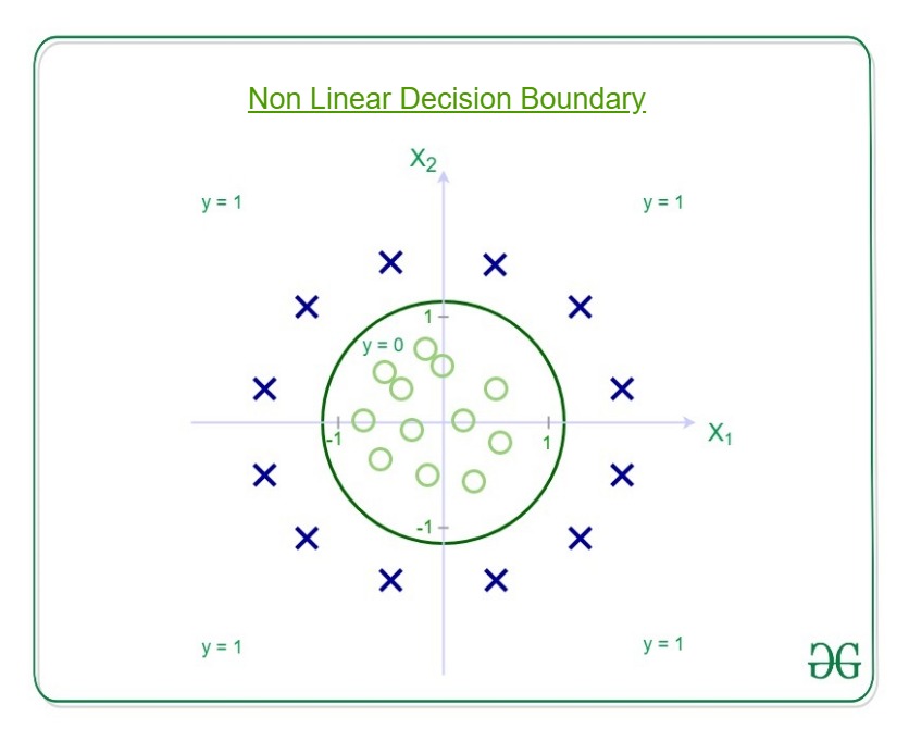
Let out weights or parameters be –

$\Theta=\begin{bmatrix} -1\\ 0\\ 0\\ 1\\ 1 \end{bmatrix}$

So, it predicts y = 1 if

$-1 + x_{1}^2 + x_{2}^2 \geqslant 0$

$\Rightarrow x_{1}^2 + x_{2}^2 \geqslant 1$

And that is the equation of a circle with radius = 1 and origin as the center. This is the Decision Boundary for our defined hypothesis.

Understanding Logistic Regression

Pre-requisite: Linear Regression
This article discusses the basics of Logistic Regression and its implementation in Python. Logistic regression is basically a supervised classification algorithm. In a classification problem, the target variable(or output), y, can take only discrete values for given set of features(or inputs), X.

Contrary to popular belief, logistic regression IS a regression model. The model builds a regression model to predict the probability that a given data entry belongs to the category numbered as “1”. Just like Linear regression assumes that the data follows a linear function, Logistic regression models the data using the sigmoid function.

$g(z) = \frac{1}{1 + e^-^z}\$

Logistic regression becomes a classification technique only when a decision threshold is brought into the picture. The setting of the threshold value is a very important aspect of Logistic regression and is dependent on the classification problem itself.

The decision for the value of the threshold value is majorly affected by the values of precision and recall. Ideally, we want both precision and recall to be 1, but this seldom is the case. In case of a Precision-Recall tradeoff we use the following arguments to decide upon the thresold:-

1. Low Precision/High Recall: In applications where we want to reduce the number of false negatives without necessarily reducing the number false positives, we choose a decision value which has a low value of Precision or high value of Recall. For example, in a cancer diagnosis application, we do not want any affected patient to be classified as not affected without giving much heed to if the patient is being wrongfully diagnosed with cancer. This is because, the absence of cancer can be detected by further medical diseases but the presence of the disease cannot be detected in an already rejected candidate.

2. High Precision/Low Recall: In applications where we want to reduce the number of false positives without necessarily reducing the number false negatives, we choose a decision value which has a high value of Precision or low value of Recall. For example, if we are classifying customers whether they will react positively or negatively to a personalised advertisement, we want to be absolutely sure that the customer will react positively to the advertisemnt because otherwise, a negative reaction can cause a loss potential sales from the customer.

Based on the number of categories, Logistic regression can be classified as:

binomial: target variable can have only 2 possible types: “0” or “1” which may represent “win” vs “loss”, “pass” vs “fail”, “dead” vs “alive”, etc.
multinomial: target variable can have 3 or more possible types which are not ordered(i.e. types have no quantitative significance) like “disease A” vs “disease B” vs “disease C”.
ordinal: it deals with target variables with ordered categories. For example, a test score can be categorized as:“very poor”, “poor”, “good”, “very good”. Here, each category can be given a score like 0, 1, 2, 3.

First of all, we explore the simplest form of Logistic Regression, i.e Binomial Logistic Regression.

Binomial Logistic Regression

Consider an example dataset which maps the number of hours of study with the result of an exam. The result can take only two values, namely passed(1) or failed(0):

HOURS(X)	0.50	0.75	1.00	1.25	1.50	1.75	2.00	2.25	2.50	2.75	3.00	3.25	3.50	3.75	4.00	4.25	4.50	4.75	5.00	5.50
PASS(Y)	0	0	0	0	0	0	1	0	1	0	1	0	1	0	1	1	1	1	1	1

So, we have
$y = \left\{\begin{matrix} 0,if fail\\ 1,if pass\\ \end{matrix}\right.$
i.e. y is a categorical target variable which can take only two possible type:“0” or “1”.
In order to generalize our model, we assume that:

The dataset has ‘p’ feature variables and ‘n’ observations.
The feature matrix is represented as:
$\mathbf{X} =\begin{pmatrix} 1 & x_{11} & \cdots & x_{1p} \\ 1 & x_{21} & \cdots & x_{2p} \\ \vdots & \vdots & \ddots & \vdots \\ 1 & x_{n1} & \cdots & x_{np} \end{pmatrix}$
Here, $x_{ij}$ denotes the values of $j^{th}$ feature for $i^{th}$ observation.
Here, we are keeping the convention of letting $x_{i0}$ = 1. (Keep reading, you will understand the logic in a few moments).
The $i^{th}$ observation, $x_i$ , can be represented as:
$x_i = \begin{bmatrix} 1\\ x_{i1}\\ x_{i2}\\ .\\ .\\ x_{ip}\\ \end{bmatrix}$
$h(x_i)$ represents the predicted response for $i^{th}$ observation, i.e. $x_i$ . The formula we use for calculating $h(x_i)$ is called hypothesis.

If you have gone though Linear Regression, you should recall that in Linear Regression, the hypothesis we used for prediction was:
$h(x_i) = \beta_0 + \beta_1x_{i1} + \beta_2x_{i2} + ..... + \beta_px_{ip}$
where, $\beta_0, \beta_1,…, \beta_p$ are the regression coefficients.
Let regression coefficient matrix/vector, $\beta$ be:
$\beta = \begin{bmatrix} \beta_0\\ \beta_1\\ \beta_2\\ .\\ .\\ \beta_p\\ \end{bmatrix}$
Then, in a more compact form,
$h(x_i) = \beta^Tx_i$

The reason for taking $x_0$ = 1 is pretty clear now.
We needed to do a matrix product, but there was no
actual $x_0$ multiplied to $\beta_0$ in original hypothesis formula. So, we defined $x_0$ = 1.

Now, if we try to apply Linear Regression on above problem, we are likely to get continuous values using the hypothesis we discussed above. Also, it does not make sense for $h(x_i)$ to take values larger that 1 or smaller than 0.
So, some modifications are made to the hypothesis for classification:
$h(x_i) = g(\beta^T x_i) = \frac{1}{1 + e^{-\beta^T x_i}}$
where,
$g(z) = \frac{1}{1 + e^{-z}}$
is called logistic function or the sigmoid function.
Here is a plot showing g(z):

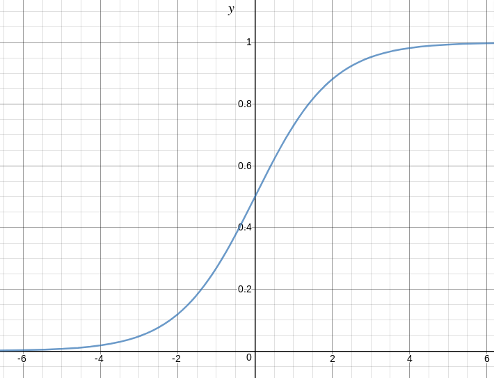
We can infer from above graph that:

g(z) tends towards 1 as $z\rightarrow\infty$
g(z) tends towards 0 as $z\rightarrow-\infty$
g(z) is always bounded between 0 and 1

So, now, we can define conditional probabilities for 2 labels(0 and 1) for $i^{th}$ observation as:
$\newline P(y_i = 1|x_i; \beta) = h(x_i) \newline P(y_i=0|x_i; \beta) = 1 - h(x_i)$
We can write it more compactly as:
$P(y_i|x_i;\beta) = (h(x_i))^{y_i}(1-h(x_i))^{1-y_i}$
Now, we define another term, likelihood of parameters as:
$\newline L(\beta) = \prod_{i=1}^{n}P(y_i|x_i;\beta) \newline or \newline L(\beta) = \prod_{i=1}^{n}(h(x_i))^{y_i}(1-h(x_i))^{1-y_i}$

Likelihood is nothing but the probability of data(training examples), given a model and specific parameter values(here, $\beta$ ). It measures the support provided by the data for each possible value of the $\beta$ . We obtain it by multiplying all $P(y_i|x_i)$ for given $\beta$ .

And for easier calculations, we take log likelihood:
$\newline l(\beta) = log(L(\beta)) \newline or \newline l(\beta) = \sum_{i=1}^{n}y_ilog(h(x_i)) + (1-y_i)log(1-h(x_i))$
The cost function for logistic regression is proportional to inverse of likelihood of parameters. Hence, we can obtain an expression for cost function, J using log likelihood equation as:
$J(\beta) =\sum_{i=1}^{n} - y_ilog(h(x_i)) - (1-y_i)log(1-h(x_i))$
and our aim is to estimate $\beta$ so that cost function is minimized !!

Using Gradient descent algorithm

Firstly, we take partial derivatives of $J(\beta)$ w.r.t each $\beta_j \in \beta$ to derive the stochastic gradient descent rule(we present only the final derived value here):
$\frac{\partial J(\beta)}{\partial \beta_j} = (h(x) - y)x_j$
Here, y and h(x) represent the response vector and predicted response vector(respectively). Also, $x_j$ is the vector representing the observation values for $j^{th}$ feature.
Now, in order to get min $J(\beta)$ ,
$\newline Repeat\{ \newline \beta_j := \beta_j - \alpha\sum_{i=1}^{n}(h(x_i)-y_i)x_{ij} \newline (Simultaneously\hspace{5}update\hspace{5}all\hspace{5}\beta_j) \newline \}$
where $\alpha$ is called learning rate and needs to be set explicitly.
Let us see the python implementation of above technique on a sample dataset (download it from here):

2.25 2.50 2.75 3.00 3.25 3.50 3.75 4.00 4.25 4.50 4.75 5.00 5.50

import csv 
import numpy as np 
import matplotlib.pyplot as plt 
def loadCSV(filename): 
''' 
function to load dataset 
'''
with open(filename,"r") as csvfile: 
lines = csv.reader(csvfile) 
dataset = list(lines) 
for i in range(len(dataset)): 
dataset[i] = [float(x) for x in dataset[i]]      
return np.array(dataset) 
def normalize(X): 
''' 
function to normalize feature matrix, X 
'''
mins = np.min(X, axis = 0) 
maxs = np.max(X, axis = 0) 
rng = maxs - mins 
norm_X = 1 - ((maxs - X)/rng) 
return norm_X 
def logistic_func(beta, X): 
''' 
logistic(sigmoid) function 
'''
return 1.0/(1 + np.exp(-np.dot(X, beta.T))) 
def log_gradient(beta, X, y): 
''' 
logistic gradient function 
'''
first_calc = logistic_func(beta, X) - y.reshape(X.shape[0], -1) 
final_calc = np.dot(first_calc.T, X) 
return final_calc 
def cost_func(beta, X, y): 
''' 
cost function, J 
'''
log_func_v = logistic_func(beta, X) 
y = np.squeeze(y) 
step1 = y * np.log(log_func_v) 
step2 = (1 - y) * np.log(1 - log_func_v) 
final = -step1 - step2 
return np.mean(final) 
def grad_desc(X, y, beta, lr=.01, converge_change=.001): 
''' 
gradient descent function 
'''
cost = cost_func(beta, X, y) 
change_cost = 1
num_iter = 1
while(change_cost > converge_change): 
old_cost = cost 
beta = beta - (lr * log_gradient(beta, X, y)) 
cost = cost_func(beta, X, y) 
change_cost = old_cost - cost 
num_iter += 1
return beta, num_iter  
def pred_values(beta, X): 
''' 
function to predict labels 
'''
pred_prob = logistic_func(beta, X) 
pred_value = np.where(pred_prob >= .5, 1, 0) 
return np.squeeze(pred_value) 
def plot_reg(X, y, beta): 
''' 
function to plot decision boundary 
'''
# labelled observations 
x_0 = X[np.where(y == 0.0)] 
x_1 = X[np.where(y == 1.0)] 
# plotting points with diff color for diff label 
plt.scatter([x_0[:, 1]], [x_0[:, 2]], c='b', label='y = 0') 
plt.scatter([x_1[:, 1]], [x_1[:, 2]], c='r', label='y = 1') 
# plotting decision boundary 
x1 = np.arange(0, 1, 0.1) 
x2 = -(beta[0,0] + beta[0,1]*x1)/beta[0,2] 
plt.plot(x1, x2, c='k', label='reg line') 
plt.xlabel('x1') 
plt.ylabel('x2') 
plt.legend() 
plt.show() 
if __name__ == "__main__": 
# load the dataset 
dataset = loadCSV('dataset1.csv') 
# normalizing feature matrix 
X = normalize(dataset[:, :-1]) 
# stacking columns wth all ones in feature matrix 
X = np.hstack((np.matrix(np.ones(X.shape[0])).T, X)) 
# response vector 
y = dataset[:, -1] 
# initial beta values 
beta = np.matrix(np.zeros(X.shape[1])) 
# beta values after running gradient descent 
beta, num_iter = grad_desc(X, y, beta) 
# estimated beta values and number of iterations 
print("Estimated regression coefficients:", beta) 
print("No. of iterations:", num_iter) 
# predicted labels 
y_pred = pred_values(beta, X) 
# number of correctly predicted labels 
print("Correctly predicted labels:", np.sum(y == y_pred)) 
# plotting regression line 
plot_reg(X, y, beta) 

Estimated regression coefficients: [[  1.70474504  15.04062212 -20.47216021]]
No. of iterations: 2612
Correctly predicted labels: 100

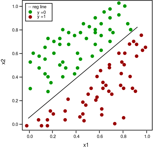
Note: Gradient descent is one of the many way to estimate $\beta$ .
Basically, these are more advanced algorithms which can be easily run in Python once you have defined your cost function and your gradients. These algorithms are:

BFGS(Broyden–Fletcher–Goldfarb–Shanno algorithm)
L-BFGS(Like BFGS but uses limited memory)
Conjugate Gradient

Advantages/disadvantages of using any one of these algorithms over Gradient descent:

Advantages
- Don’t need to pick learning rate
- Often run faster (not always the case)
- Can numerically approximate gradient for you (doesn’t always work out well)
Disadvantages
- More complex
- More of a black box unless you learn the specifics

Multinomial Logistic Regression

In Multinomial Logistic Regression, the output variable can have more than two possible discrete outputs. Consider the Digit Dataset. Here, the output variable is the digit value which can take values out of (0, 12, 3, 4, 5, 6, 7, 8, 9).
Given below is the implementation of Multinomial Logisitc Regression using scikit-learn to make predictions on digit dataset.

from sklearn import datasets, linear_model, metrics 
# load the digit dataset 
digits = datasets.load_digits() 
# defining feature matrix(X) and response vector(y) 
X = digits.data 
y = digits.target 
# splitting X and y into training and testing sets 
from sklearn.model_selection import train_test_split 
X_train, X_test, y_train, y_test = train_test_split(X, y, test_size=0.4, 
random_state=1) 
# create logistic regression object 
reg = linear_model.LogisticRegression() 
# train the model using the training sets 
reg.fit(X_train, y_train) 
# making predictions on the testing set 
y_pred = reg.predict(X_test) 
# comparing actual response values (y_test) with predicted response values (y_pred) 
print("Logistic Regression model accuracy(in %):",  
metrics.accuracy_score(y_test, y_pred)*100) 

Logistic Regression model accuracy(in %): 95.6884561892

At last, here are some points about Logistic regression to ponder upon:

Does NOT assume a linear relationship between the dependent variable and the independent variables, but it does assume linear relationship between the logit of the explanatory variables and the response.
Independent variables can be even the power terms or some other nonlinear transformations of the original independent variables.
The dependent variable does NOT need to be normally distributed, but it typically assumes a distribution from an exponential family (e.g. binomial, Poisson, multinomial, normal,…); binary logistic regression assume binomial distribution of the response.
The homogeneity of variance does NOT need to be satisfied.
Errors need to be independent but NOT normally distributed.
It uses maximum likelihood estimation (MLE) rather than ordinary least squares (OLS) to estimate the parameters, and thus relies on large-sample approximations.

References:

ML | Logistic Regression using Python

Prerequisite: Understanding Logistic Regression

User Database – This dataset contains information of users from a companies database. It contains information about UserID, Gender, Age, EstimatedSalary, Purchased. We are using this dataset for predicting that a user will purchase the company’s newly launched product or not.

Data – User_Data

Let’s make the Logistic Regression model, predicting whether a user will purchase the product or not.

Inputing Libraries

filter_nonebrightness_4

import pandas as pd 
import numpy as np 
import matplotlib.pyplot as plt

Loading dataset – User_Data

filter_nonebrightness_4

dataset = pd.read_csv('...\\User_Data.csv')

Now, to predict whether a user will purchase the product or not, one needs to find out the relationship between Age and Estimated Salary. Here User ID and Gender are not important factors for finding out this.

filter_nonebrightness_4

# input 
x = dataset.iloc[:, [2, 3]].values 
 
# output 
y = dataset.iloc[:, 4].values

Splitting the dataset to train and test. 75% of data is used for training the model and 25% of it is used to test the performance of our model.

filter_nonebrightness_4

from sklearn.cross_validation import train_test_split 
xtrain, xtest, ytrain, ytest = train_test_split( 
        x, y, test_size = 0.25, random_state = 0)

Now, it is very important to perform feature scaling here because Age and Estimated Salary values lie in different ranges. If we don’t scale the features then Estimated Salary feature will dominate Age feature when the model finds the nearest neighbor to a data point in data space.

filter_nonebrightness_4



from sklearn.preprocessing import StandardScaler 
sc_x = StandardScaler() 
xtrain = sc_x.fit_transform(xtrain)  
xtest = sc_x.transform(xtest) 
 
print (xtrain[0:10, :]) 

Output :

[[ 0.58164944 -0.88670699]
 [-0.60673761  1.46173768]
 [-0.01254409 -0.5677824 ]
 [-0.60673761  1.89663484]
 [ 1.37390747 -1.40858358]
 [ 1.47293972  0.99784738]
 [ 0.08648817 -0.79972756]
 [-0.01254409 -0.24885782]
 [-0.21060859 -0.5677824 ]
 [-0.21060859 -0.19087153]]

Here once see that Age and Estimated salary features values are sacled and now there in the -1 to 1. Hence, each feature will contribute equally in decision making i.e. finalizing the hypothesis.

Finally, we are training our Logistic Regression model.

filter_nonebrightness_4

from sklearn.linear_model import LogisticRegression 
classifier = LogisticRegression(random_state = 0) 
classifier.fit(xtrain, ytrain)

After training the model, it time to use it to do prediction on testing data.

filter_nonebrightness_4

y_pred = classifier.predict(xtest)

Let’s test the performance of our model – Confusion Matrix

filter_nonebrightness_4

from sklearn.metrics import confusion_matrix 
cm = confusion_matrix(ytest, y_pred) 
 
print ("Confusion Matrix : \n", cm)

Output :

Confusion Matrix : 
 [[65  3]
 [ 8 24]]

Out of 100 :
TruePostive + TrueNegative = 65 + 24
FalsePositive + FalseNegative = 3 + 8

Performance measure – Accuracy

filter_nonebrightness_4

from sklearn.metrics import accuracy_score 
print ("Accuracy : ", accuracy_score(ytest, y_pred))

Output :

Accuracy :  0.89

Visualizing the performance of our model.

filter_nonebrightness_4



from matplotlib.colors import ListedColormap 
X_set, y_set = xtest, ytest 
X1, X2 = np.meshgrid(np.arange(start = X_set[:, 0].min() - 1,  
                               stop = X_set[:, 0].max() + 1, step = 0.01), 
                     np.arange(start = X_set[:, 1].min() - 1,  
                               stop = X_set[:, 1].max() + 1, step = 0.01)) 
 
plt.contourf(X1, X2, classifier.predict( 
             np.array([X1.ravel(), X2.ravel()]).T).reshape( 
             X1.shape), alpha = 0.75, cmap = ListedColormap(('red', 'green'))) 
 
plt.xlim(X1.min(), X1.max()) 
plt.ylim(X2.min(), X2.max()) 
 
for i, j in enumerate(np.unique(y_set)): 
    plt.scatter(X_set[y_set == j, 0], X_set[y_set == j, 1], 
                c = ListedColormap(('red', 'green'))(i), label = j) 
     
plt.title('Classifier (Test set)') 
plt.xlabel('Age') 
plt.ylabel('Estimated Salary') 
plt.legend() 
plt.show() 

Output :

Analysing the performance measures – accuracy and confusion matrix and the graph, we can clearly say that our model is performing really good.