Multiple linear regression

Multiple linear regression attempts to model the relationship between two or more features and a response by fitting a linear equation to observed data.

Clearly, it is nothing but an extension of Simple linear regression.

Consider a dataset with p features(or independent variables) and one response(or dependent variable).
Also, the dataset contains n rows/observations.

We define:

X (feature matrix) = a matrix of size n X p where x_{ij} denotes the values of jth feature for ith observation.

So,
$\begin{pmatrix} x_{11} & \cdots & x_{1p} \\ x_{21} & \cdots & x_{2p} \\ \vdots & \ddots & \vdots \\ x_{n1} & \vdots & x_{np} \end{pmatrix}$

and

y (response vector) = a vector of size n where y_{i} denotes the value of response for ith observation.

$y = \begin{bmatrix} y_1\\ y_2\\ .\\ .\\ y_n \end{bmatrix}$

The regression line for p features is represented as:
$h(x_i) = \beta_0 + \beta_1x_{i1} + \beta_2x_{i2} + .... + \beta_px_{ip}$
where h(x_i) is predicted response value for ith observation and b_0, b_1, …, b_p are the regression coefficients.

Also, we can write:
$\newline y_i = \beta_0 + \beta_1x_{i1} + \beta_2x_{i2} + .... + \beta_px_{ip} + \varepsilon_i \newline or \newline y_i = h(x_i) + \varepsilon_i \Rightarrow \varepsilon_i = y_i - h(x_i)$

where e_i represents residual error in ith observation.

We can generalize our linear model a little bit more by representing feature matrix X as:
$X = \begin{pmatrix} 1 & x_{11} & \cdots & x_{1p} \\ 1 & x_{21} & \cdots & x_{2p} \\ \vdots & \vdots & \ddots & \vdots \\ 1 & x_{n1} & \cdots & x_{np} \end{pmatrix}$
So now, the linear model can be expressed in terms of matrices as:
$y = X\beta + \varepsilon$

where,
$\beta = \begin{bmatrix} \beta_0\\ \beta_1\\ .\\ .\\ \beta_p \end{bmatrix}$

and

$\varepsilon = \begin{bmatrix} \varepsilon_1\\ \varepsilon_2\\ .\\ .\\ \varepsilon_n \end{bmatrix}$

Now, we determine estimate of b, i.e. b’ using Least Squares method.

As already explained, Least Squares method tends to determine b’ for which total residual error is minimized.

We present the result directly here:
$\hat{\beta} = ({X}'X)^{-1} {X}'y$
where ‘ represents the transpose of the matrix while -1 represents the matrix inverse.

Knowing the least square estimates, b’, the multiple linear regression model can now be estimated as:

$\hat{y} = X\hat{\beta}$

where y’ is estimated response vector.

Note: The complete derivation for obtaining least square estimates in multiple linear regression can be found here.

Given below is the implementation of multiple linear regression technique on the Boston house pricing dataset using Scikit-learn.

import matplotlib.pyplot as plt
import numpy as np
from sklearn import datasets, linear_model, metrics
 
# load the boston dataset
boston = datasets.load_boston(return_X_y=False)
 
# defining feature matrix(X) and response vector(y)
X = boston.data
y = boston.target
 
# splitting X and y into training and testing sets
from sklearn.model_selection import train_test_split
X_train, X_test, y_train, y_test = train_test_split(X, y, test_size=0.4,
                                                    random_state=1)
 
# create linear regression object
reg = linear_model.LinearRegression()
 
# train the model using the training sets
reg.fit(X_train, y_train)
 
# regression coefficients
print('Coefficients: \n', reg.coef_)
 
# variance score: 1 means perfect prediction
print('Variance score: {}'.format(reg.score(X_test, y_test)))
 
# plot for residual error
 
## setting plot style
plt.style.use('fivethirtyeight')
 
## plotting residual errors in training data
plt.scatter(reg.predict(X_train), reg.predict(X_train) - y_train,
            color = "green", s = 10, label = 'Train data')
 
## plotting residual errors in test data
plt.scatter(reg.predict(X_test), reg.predict(X_test) - y_test,
            color = "blue", s = 10, label = 'Test data')
 
## plotting line for zero residual error
plt.hlines(y = 0, xmin = 0, xmax = 50, linewidth = 2)
 
## plotting legend
plt.legend(loc = 'upper right')
 
## plot title
plt.title("Residual errors")
 
## function to show plot
plt.show()

Output of above program looks like this:

Coefficients:
[ -8.80740828e-02   6.72507352e-02   5.10280463e-02   2.18879172e+00
-1.72283734e+01   3.62985243e+00   2.13933641e-03  -1.36531300e+00
2.88788067e-01  -1.22618657e-02  -8.36014969e-01   9.53058061e-03
-5.05036163e-01]
Variance score: 0.720898784611

and Residual Error plot looks like this:

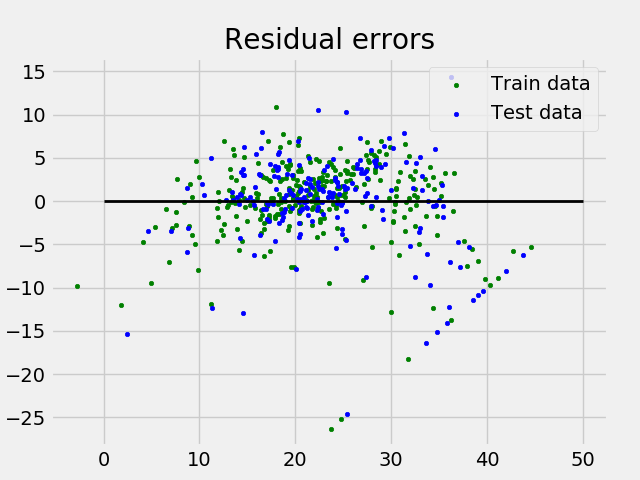
In above example, we determine accuracy score using Explained Variance Score.
We define:
explained_variance_score = 1 – Var{y – y’}/Var{y}
where y’ is the estimated target output, y the corresponding (correct) target output, and Var is Variance, the square of the standard deviation.
The best possible score is 1.0, lower values are worse.

Assumptions

Given below are the basic assumptions that a linear regression model makes regarding a dataset on which it is applied:

Linear relationship: Relationship between response and feature variables should be linear. The linearity assumption can be tested using scatter plots. As shown below, 1st figure represents linearly related variables where as variables in 2nd and 3rd figure are most likely non-linear. So, 1st figure will give better predictions using linear regression.
Little or no multi-collinearity: It is assumed that there is little or no multicollinearity in the data. Multicollinearity occurs when the features (or independent variables) are not independent from each other.
Little or no auto-correlation: Another assumption is that there is little or no autocorrelation in the data. Autocorrelation occurs when the residual errors are not independent from each other. You can refer here for more insight into this topic.
Homoscedasticity: Homoscedasticity describes a situation in which the error term (that is, the “noise” or random disturbance in the relationship between the independent variables and the dependent variable) is the same across all values of the independent variables. As shown below, figure 1 has homoscedasticity while figure 2 has heteroscedasticity.

As we reach to the end of this article, we discuss some applications of linear regression below.

Applications:

1. Trend lines: A trend line represents the variation in some quantitative data with passage of time (like GDP, oil prices, etc.). These trends usually follow a linear relationship. Hence, linear regression can be applied to predict future values. However, this method suffers from a lack of scientific validity in cases where other potential changes can affect the data.

2. Economics: Linear regression is the predominant empirical tool in economics. For example, it is used to predict consumption spending, fixed investment spending, inventory investment, purchases of a country’s exports, spending on imports, the demand to hold liquid assets, labor demand, and labor supply.

3. Finance: Capital price asset model uses linear regression to analyze and quantify the systematic risks of an investment.

4. Biology: Linear regression is used to model causal relationships between parameters in biological systems.

References:

ML | Multiple Linear Regression using Python

Linear Regression:
It is the basic and commonly used type for predictive analysis. It is a statistical approach to modeling the relationship between a dependent variable and a given set of independent variables.

These are of two types:

Simple linear Regression
Multiple Linear Regression

Let’s Discuss Multiple Linear Regression using Python.

Multiple Linear Regression attempts to model the Relationship between two or more features and a response by fitting a linear equation to observed data. The steps to perform multiple linear Regression are almost similar to that of simple linear Regression. The Difference Lies in the Evalution. We can use it to find out which factor has the highest impact on the predicted output and now different variable relate to each other.

Here : Y= b0 + b1*x1 + b2*x2 + b3*x3 +…… bn*xn
Y = Dependent variable and x1, x2, x3, …… xn = multiple independent variables

Assumption of Regression Model :

Linearity: The relationship between dependent and independent variables should be linear.
Homoscedasticity: Constant variance of the errors should be maintained.
Multivariate normality: Multiple Regression assumes that the residuals are normally distributed.
Lack of Multicollinearity: It is assumed that there is little or no multicollinearity in the data.

Dummy Variable –
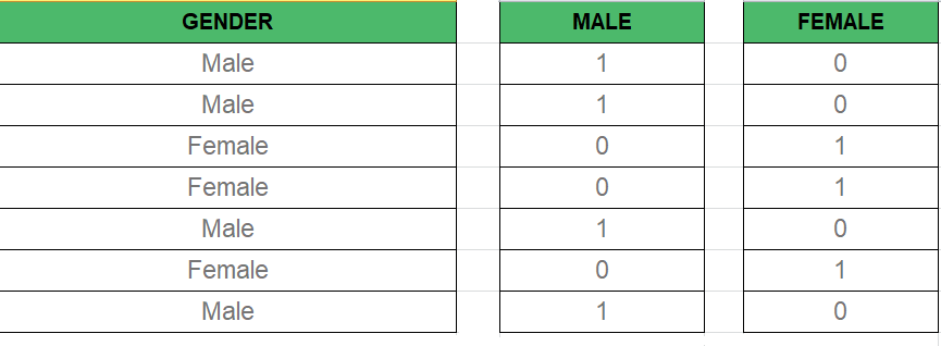
As we Know in the Multiple Regression Model we use a lot of categorical data. Using Categorical Data is a good method to include non-numeric data into respective Regression Model. Categorical Data refers to data values which represent categories-data values with fixed and unordered number of values, for instance, gender(male/female). In the regression model, these values can be represented by Dummy Variables.

These variable consist of values such as 0 or 1 representing the presence and absence of categorical value.

Dummy Variable Trap –
The Dummy Variable Trap is a condition in which two or more are Highly Correlated. In the simple term, we can say that one variable can be predicted from the prediction of the other. The solution of the Dummy Variable Trap is to drop one the categorical variable. So if there are m Dummy variables then m-1 variables are used in the model.

 D2= D1-1   
 Here D2, D1 = Dummy Variables

Method of Building Models :

All-in
Backward-Elimination
Forward Selection
Bidirectional Elimination
Score Comparison

Backward-Elimination :

Step #1 : Select a significant level to start in the model.
Step #2 : Fit the full model with all possible predictor.
Step #3 : Consider the predictor with highest P-value. If P > SL go to STEP 4, otherwise model is Ready.
Step #4 : Remove the predictor.
Step #5 : Fit the model without this variable.

Forward-Selection :

Step #1 : Select a significance level to enter the model(e.g. SL = 0.05)
Step #2 : Fit all simple regression models y~ x(n). Select the one with the lowest P-value .
Step #3 : Keep this variable and fit all possible models with one extra predictor added to the one(s) you already have.
Step #4 : Consider the predictor with lowest P-value. If P < SL, go to Step #3, otherwise model is Ready.

Steps Involved in any Multiple Linear Regression Model

Step #1: Data Pre Processing
a) Importing The Libraries.
b) Importing the Data Set.
c) Encoding the Categorical Data.
d) Avoiding the Dummy Variable Trap.
e) Splitting the Data set into Training Set and Test Set.

Step #2: Fitting Multiple Linear Regression to the Training set
Step #3: Predicting the Test set results.

Code #1 :

filter_nonebrightness_4



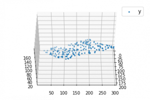
import numpy as np 
import matplotlib as mpl 
from mpl_toolkits.mplot3d import Axes3D 
import matplotlib.pyplot as plt 
def generate_dataset(n): 
x = [] 
y = [] 
random_x1 = np.random.rand() 
random_x2 = np.random.rand() 
for i in range(n): 
x1 = i 
x2 = i/2 + np.random.rand()*n 
x.append([1, x1, x2]) 
y.append(random_x1 * x1 + random_x2 * x2 + 1) 
return np.array(x), np.array(y) 
x, y = generate_dataset(200) 
mpl.rcParams['legend.fontsize'] = 12
fig = plt.figure() 
ax = fig.gca(projection ='3d') 
ax.scatter(x[:, 1], x[:, 2], y, label ='y', s = 5) 
ax.legend() 
ax.view_init(45, 0) 
plt.show() 

Output:

Code #2:

filter_nonebrightness_4



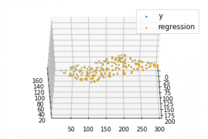
def mse(coef, x, y): 
return np.mean((np.dot(x, coef) - y)**2)/2
def gradients(coef, x, y): 
return np.mean(x.transpose()*(np.dot(x, coef) - y), axis = 1) 
def multilinear_regression(coef, x, y, lr, b1 = 0.9, b2 = 0.999, epsilon = 1e-8): 
prev_error = 0
m_coef = np.zeros(coef.shape) 
v_coef = np.zeros(coef.shape) 
moment_m_coef = np.zeros(coef.shape) 
moment_v_coef = np.zeros(coef.shape) 
t = 0
while True: 
error = mse(coef, x, y) 
if abs(error - prev_error) <= epsilon: 
break
prev_error = error 
grad = gradients(coef, x, y) 
t += 1
m_coef = b1 * m_coef + (1-b1)*grad 
v_coef = b2 * v_coef + (1-b2)*grad**2
moment_m_coef = m_coef / (1-b1**t) 
moment_v_coef = v_coef / (1-b2**t) 
delta = ((lr / moment_v_coef**0.5 + 1e-8) *
(b1 * moment_m_coef + (1-b1)*grad/(1-b1**t))) 
coef = np.subtract(coef, delta) 
return coef 
coef = np.array([0, 0, 0]) 
c = multilinear_regression(coef, x, y, 1e-1) 
fig = plt.figure() 
ax = fig.gca(projection ='3d') 
ax.scatter(x[:, 1], x[:, 2], y, label ='y', 
s = 5, color ="dodgerblue") 
ax.scatter(x[:, 1], x[:, 2], c[0] + c[1]*x[:, 1] + c[2]*x[:, 2], 
label ='regression', s = 5, color ="orange") 
ax.view_init(45, 0) 
ax.legend() 
plt.show() 

Output:

ML | Multiple Linear Regression (Backward Elimination Technique)

Multiple Linear Regression is a type of regression where the model depends on several independent variables(instead of only on one independent variable as seen in the case of Simple Linear Regression). Multiple Linear Regression has several techniques to build an effective model namely:-

All-in
Backward Elimination
Forward Selection
Bidirectional Elimination

In this article, we will implement multiple linear regression using the backward elimination technique.
Backward Elimination consists of the following steps:

Select a significance level to stay in the model (eg. SL = 0.05)
Fit the model with all possible predictors
Consider the predictor with the highest P-value. If P>SL, go to point d.
Remove the predictor
Fit the model without this variable and repeat the step c until the condition becomes false.

Let us suppose that we have a dataset containing a set of expenditure information for different companies. We would like to know the profit made by each company to determine which company can give the best results if collaborated with them. We build the regression model using a step by step approach.

Step 1 : Basic preprocessing and encoding

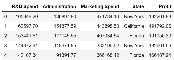
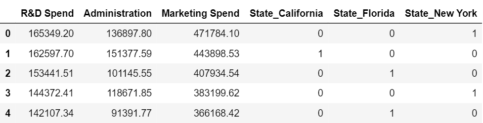
# import the necessary libraries 
import pandas as pd 
import numpy as np 
from sklearn.model_selection import train_test_split 
# import the dataset 
df = pd.read_csv('50_Startups.csv') 
# first five entries of the dataset 
df.head() 
# split the dataframe into dependent and independent variables.  
x = df[['R&D Spend', 'Administration', 'Marketing Spend', 'State']] 
y = df['Profit'] 
x.head() 
y.head() 
# since the state is a string datatype column we need to encode it. 
x = pd.get_dummies(x) 
x.head() 

Dataset

The set of independent variables after encoding the state column

Step 2 : Splitting the data into training and testing set and making predictions

x_train, x_test, y_train, y_test = train_test_split( 
x, y, test_size = 0.3, random_state = 0) 
from sklearn.linear_model import LinearRegression 
lm = LinearRegression() 
lm.fit(x_train, y_train) 
pred = lm.predict(x_test) 

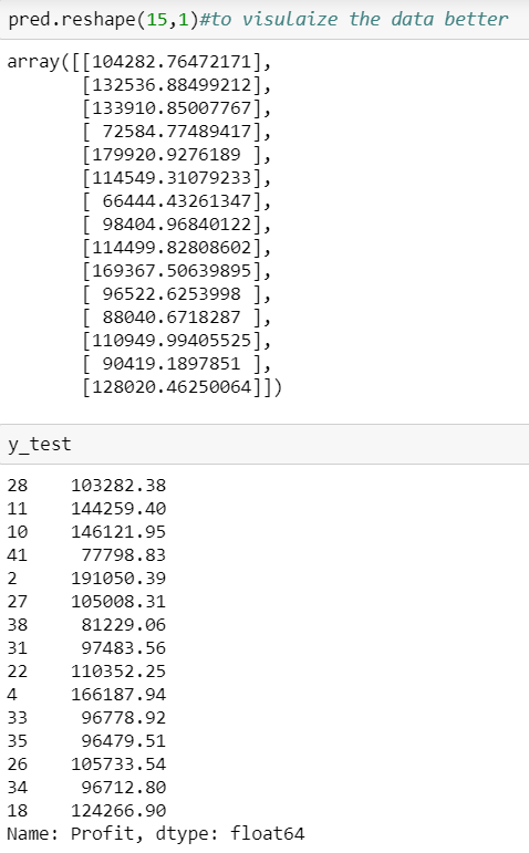
We can see that our predictions our close enough to the test set but how do we find the most important factor contributing to the profit.
Here is a solution for that.
We know that the equation of a mutliple linear regression line is given by y=b1+b2*x+b3*x’+b4*x”+…….
where b1, b2, b3, … are the coefficients and x, x’, x” are all independent variables.
Since we dont have any ‘x’ for the first coefficient we assume it can be written as a product of b and 1 and hence we append a column of ones. There are libraries that take care of it but since we are using the stats model library we need to explicitly add the column.
Step 3 : Using the backward elimination technique

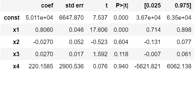
import statsmodels.formula.api as sm 
# add a column of ones as integer data type 
x = np.append(arr = np.ones((50, 1)).astype(int),  
values = x, axis = 1) 
# choose a Significance level usually 0.05, if p>0.05 
#  for the highest values parameter, remove that value 
x_opt = x[:, [0, 1, 2, 3, 4, 5]] 
ols = sm.OLS(endog = y, exog = x_opt).fit() 
ols.summary() 

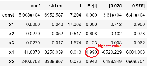
This figure shows the highest valued parameter

And now we follow the steps of the backward elimination and start eliminating unnecessary parameters.

# remove the 4th column as it has the highest value 
x_opt = x[:, [0, 1, 2, 3, 5]] 
ols = sm.OLS(endog = y, exog = x_opt).fit() 
ols.summary() 
# remove the 5th column as it has the highest value 
x_opt = x[:, [0, 1, 2, 3]] 
ols = sm.OLS(endog = y, exog = x_opt).fit() 
ols.summary() 
# remove the 3rd column as it has the highest value 
x_opt = x[:, [0, 1, 2]] 
ols = sm.OLS(endog = y, exog = x_opt).fit() 
ols.summary() 
# remove the 2nd column as it has the highest value 
x_opt = x[:, [0, 1]] 
ols = sm.OLS(endog = y, exog = x_opt).fit() 
ols.summary() 

Summary after removing the first unnecessary parameter.

So if we continue the process we see that we are left with only one column at the end and that is the R&D spent.We can conclude that the company which has maximum expenditure on the R&D makes the highest profit.

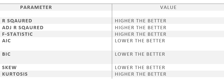
With this, we have solved the problem statement of finding the company for collaboration. Now let us have a brief look at the parameters of the OLS summary.

- R square – It tells about the goodness of the fit. It ranges between 0 and 1. The closer the value to 1, the better it is. It explains the extent of variation of the dependent variables in the model. However, it is biased in a way that it never decreases(even on adding variables).
- Adj Rsquare – This parameter has a penalising factor(the no. of regressors) and it always decreases or stays identical to the previous value as the number of independent variables increases. If its value keeps increasing on removing the unnecessary parameters go ahead with the model or stop and revert.
- F statistic – It is used to compare two variances and is always greater than 0. It is formulated as v1²/v2². In regression, it is the ratio of the explained to the unexplained variance of the model.
- AIC and BIC – AIC stands for Akaike’s information criterion and BIC stands for Bayesian information criterion Both these parameters depend on the likelihood function L.
- Skew – Informs about the data symmetry about the mean.
- Kurtosis – It measures the shape of the distribution i.e.the amount of data close to the mean than far away from the mean.
- Omnibus – D’Angostino’s test. It provides a combined statistical test for the presence of skewness and kurtosis.
- Log-likelihood – It is the log of the likelihood function.

######################################################

# Multiple Linear Regression

# Importing the libraries
import numpy as np
import matplotlib.pyplot as plt
import pandas as pd

# Importing the dataset
dataset = pd.read_csv('50_Startups.csv')
X = dataset.iloc[:, :-1]
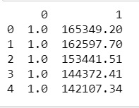
y = dataset.iloc[:, 4]

print(dataset)
#Convert the column into categorical columns

states=pd.get_dummies(X['State'],drop_first=True)

print(states)
# Drop the state coulmn
X=X.drop('State',axis=1)

# concat the dummy variables
X=pd.concat([X,states],axis=1)

# Splitting the dataset into the Training set and Test set
from sklearn.model_selection import train_test_split
X_train, X_test, y_train, y_test = train_test_split(X, y, test_size = 0.2, random_state = 0)

print("Training Set")
print(X_train)
print(y_train)

print("test set")
print(X_test)

# Fitting Multiple Linear Regression to the Training set
from sklearn.linear_model import LinearRegression
regressor = LinearRegression()
regressor.fit(X_train, y_train)