Python | Implementation of Polynomial Regression

Polynomial Regression is a form of linear regression in which the relationship between the independent variable x and dependent variable y is modeled as an nth degree polynomial. Polynomial regression fits a nonlinear relationship between the value of x and the corresponding conditional mean of y, denoted E(y |x)

Why Polynomial Regression:

There are some relationships that a researcher will hypothesize is curvilinear. Clearly, such type of cases will include a polynomial term.
Inspection of residuals. If we try to fit a linear model to curved data, a scatter plot of residuals (Y axis) on the predictor (X axis) will have patches of many positive residuals in the middle. Hence in such situation it is not appropriate.
An assumption in usual multiple linear regression analysis is that all the independent variables are independent. In polynomial regression model, this assumption is not satisfied.

Uses of Polynomial Regression:
These are basically used to define or describe non-linear phenomenon such as:

Growth rate of tissues.
Progression of disease epidemics
Distribution of carbon isotopes in lake sediments

The basic goal of regression analysis is to model the expected value of a dependent variable y in terms of the value of an independent variable x. In simple regression, we used following equation –

y = a + bx + e

Here y is dependent variable, a is y intercept, b is the slope and e is the error rate.

In many cases, this linear model will not work out For example if we analyzing the production of chemical synthesis in terms of temperature at which the synthesis take place in such cases we use quadratic model

y = a + b1x + b2^2 + e

Here y is dependent variable on x, a is y intercept and e is the error rate.

In general, we can model it for nth value.

y = a + b1x + b2x^2 +....+ bnx^n

Since regression function is linear in terms of unknown variables, hence these models are linear from the point of estimation.

Hence through Least Square technique, let’s compute the response value that is y.

Polynomial Regression in Python:
To get the Dataset used for analysis of Polynomial Regression, click here.

Step 1: Import libraries and dataset
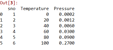
Import the important libraries and the dataset we are using to perform Polynomial Regression.

filter_nonebrightness_4



# Importing the libraries 
import numpy as np 
import matplotlib.pyplot as plt 
import pandas as pd 
# Importing the dataset 
datas = pd.read_csv('data.csv') 
datas 

Step 2: Dividing the dataset into 2 components

Divide dataset into two components that is X and y.X will contain the Column between 1 and 2. y will contain the 2 column.

filter_nonebrightness_4

X = datas.iloc[:, 1:2].values 
y = datas.iloc[:, 2].values

Step 3: Fitting Linear Regression to the dataset

Fitting the linear Regression model On two components.

filter_nonebrightness_4



# Fitting Linear Regression to the dataset 
from sklearn.linear_model import LinearRegression 
lin = LinearRegression() 
lin.fit(X, y) 

Step 4: Fitting Polynomial Regression to the dataset

Fitting the Polynomial Regression model on two components X and y.

filter_nonebrightness_4



# Fitting Polynomial Regression to the dataset 
from sklearn.preprocessing import PolynomialFeatures 
poly = PolynomialFeatures(degree = 4) 
X_poly = poly.fit_transform(X) 
poly.fit(X_poly, y) 
lin2 = LinearRegression() 
lin2.fit(X_poly, y) 

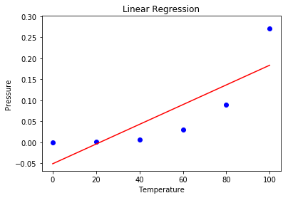
Step 5: In this step we are Visualising the Linear Regression results using scatter plot.

filter_nonebrightness_4



# Visualising the Linear Regression results 
plt.scatter(X, y, color = 'blue') 
plt.plot(X, lin.predict(X), color = 'red') 
plt.title('Linear Regression') 
plt.xlabel('Temperature') 
plt.ylabel('Pressure') 
plt.show() 

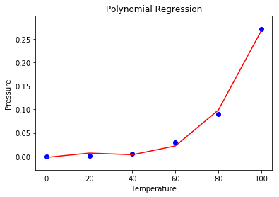
Step 6: Visualising the Polynomial Regression results using scatter plot.

filter_nonebrightness_4



# Visualising the Polynomial Regression results 
plt.scatter(X, y, color = 'blue') 
plt.plot(X, lin2.predict(poly.fit_transform(X)), color = 'red') 
plt.title('Polynomial Regression') 
plt.xlabel('Temperature') 
plt.ylabel('Pressure') 
plt.show() 

Step 7: Predicting new result with both Linear and Polynomial Regression.

filter_nonebrightness_4

# Predicting a new result with Linear Regression 
lin.predict(110.0)

filter_nonebrightness_4

# Predicting a new result with Polynomial Regression 
lin2.predict(poly.fit_transform(110.0))

Advantages of using Polynomial Regression:

Broad range of function can be fit under it.
Polynomial basically fits wide range of curvature.
Polynomial provides the best approximation of the relationship between dependent and independent variable.

Disadvantages of using Polynomial Regression

These are too sensitive to the outliers.
The presence of one or two outliers in the data can seriously affect the results of a nonlinear analysis.
In addition there are unfortunately fewer model validation tools for the detection of outliers in nonlinear regression than there are for linear regression.

Python | Finding Solutions of a Polynomial Equation

Given a quadratic equation, the task is to find the possible solutions to it.

Examples:

Input : 
enter the coef of x2 : 1
enter the coef of x  : 2
enter the costant    : 1
Output :
the value for x is -1.0

Input :
enter the coef of x2 : 2
enter the coef of x  : 3
enter the costant    : 2
Output :
x1 = -3+5.656854249492381i/4 and x2 = -3-5.656854249492381i/4

Algorithm :

Start.
Prompt the values for a, b, c. 
Compute i = b**2-4*a*c
If i get negative value g=square root(-i)
Else h = sqrt(i)
Compute e = -b+h/(2*a)
Compute f = -b-h/(2*a)
If condition e==f then
    Print e
Else
    Print e and f
If i is negative then
    Print -b+g/(2*a) and -b-g/(2*a)
stop

Below is the Python implementation of the above mentioned task.

# Python program for solving a quadratic equation. 
  
from math import sqrt    
try:      
 
    # if user gives non int values it will go to except block 
    a = 1
    b = 2
    c = 1
    i = b**2-4 * a * c 
 
    # magic condition for complex values 
    g = sqrt(-i) 
    try: 
        d = sqrt(i) 
        # two resultants 
        e = (-b + d) / 2 * a   
        f = (-b-d) / 2 * a 
        if e == f: 
            print("the values for x is " + str(e)) 
        else: 
            print("the value for x1 is " + str(e) +
                  " and x2 is " + str(f)) 
    except ValueError: 
        print("the result for your equation is in complex") 
         
        # to print complex resultants. 
        print("x1 = " + str(-b) + "+" + str(g) + "i/" + str(2 * a) +
              " and x2 = " + str(-b) + "-" + str(g) + "i/" +
              str(2 * a))    
         
except ValueError: 
    print("enter a number not a string or char") 

Output :

the values for x is -1.0

Explanation :
First, this program will get three inputs from the user. The values are the coefficient of $x2$ , coefficient of $x$ and constant. Then it performs the formula
$(-b + (or) - sqrt(b2 - 4 * a * c) / 2a)$
For complex the value of $(b2 - 4 * a * c)$ gets negative. Rooting negative values will throw a value error. In this case, turn the result of $-(b2 - 4 * a * c)$ and then root it. Don’t forget to include $i$ at last.