Creating a simple machine learning model

Create a Linear Regression Model in Python using a randomly created data set.

Linear Regression Model
Linear regression geeks for geeks

Generating the Training Set

# python library to generate random numbers 
from random import randint 
 
# the limit within which random numbers are generated 
TRAIN_SET_LIMIT = 1000
 
# to create exactly 100 data items 
TRAIN_SET_COUNT = 100
 
# list that contains input and corresponding output 
TRAIN_INPUT = list() 
TRAIN_OUTPUT = list() 
 
# loop to create 100 data  items with three columns each 
for i in range(TRAIN_SET_COUNT): 
    a = randint(0, TRAIN_SET_LIMIT) 
    b = randint(0, TRAIN_SET_LIMIT) 
    c = randint(0, TRAIN_SET_LIMIT) 
 
# creating the output for each data item 
    op = a + (2 * b) + (3 * c) 
    TRAIN_INPUT.append([a, b, c]) 
 
# adding each output to output list 
    TRAIN_OUTPUT.append(op) 

Machine Learning Model – Linear Regression

The Model can be created in two steps:-
1. Training the model with Training Data
2. Testing the model with Test Data

Training the Model
The data that was created using the above code is used to train the model

# Sk-Learn contains the linear regression model 
from sklearn.linear_model import LinearRegression 
 
# Initialize the linear regression model 
predictor = LinearRegression(n_jobs =-1) 
 
# Fill the Model with the Data 
predictor.fit(X = TRAIN_INPUT, y = TRAIN_OUTPUT) 

Testing the Data
The testing is done Manually. Testing can be done using some random data and testing if the model gives the correct result for the input data.

# Random Test data 
X_TEST = [[ 10, 20, 30 ]] 
 
# Predict the result of X_TEST which holds testing data 
outcome = predictor.predict(X = X_TEST) 
 
# Predict the coefficients 
coefficients = predictor.coef_ 
 
# Print the result obtained for the test data 
print('Outcome : {}\nCoefficients : {}'.format(outcome, coefficients)) 

The Outcome of the above provided test-data should be, 10 + 20*2 + 30*3 = 140.
Output

Outcome : [ 140.]
Coefficients : [ 1. 2. 3.]

Linear Regression (Python Implementation)

This article discusses the basics of linear regression and its implementation in Python programming language.

Linear regression is a statistical approach for modelling relationship between a dependent variable with a given set of independent variables.

Note: In this article, we refer dependent variables as response and independent variables as features for simplicity.

In order to provide a basic understanding of linear regression, we start with the most basic version of linear regression, i.e. Simple linear regression.

Simple Linear Regression

Simple linear regression is an approach for predicting a response using a single feature.

It is assumed that the two variables are linearly related. Hence, we try to find a linear function that predicts the response value(y) as accurately as possible as a function of the feature or independent variable(x).

Let us consider a dataset where we have a value of response y for every feature x:

For generality, we define:

x as feature vector, i.e x = [x_1, x_2, …., x_n],

y as response vector, i.e y = [y_1, y_2, …., y_n]

for n observations (in above example, n=10).

A scatter plot of above dataset looks like:-

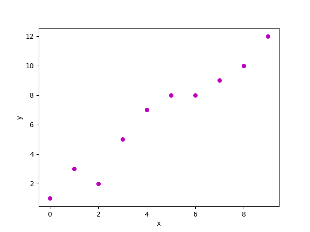
Now, the task is to find a line which fits best in above scatter plot so that we can predict the response for any new feature values. (i.e a value of x not present in dataset)

This line is called regression line.

The equation of regression line is represented as:

$h(x_i) = \beta _0 + \beta_1x_i$

Here,

h(x_i) represents the predicted response value for ith observation.
b_0 and b_1 are regression coefficients and represent y-intercept and slope of regression line respectively.

To create our model, we must “learn” or estimate the values of regression coefficients b_0 and b_1. And once we’ve estimated these coefficients, we can use the model to predict responses!

In this article, we are going to use the Least Squares technique.

Now consider:

$y_i = \beta_0 + \beta_1x_i + \varepsilon_i = h(x_i) + \varepsilon_i \Rightarrow \varepsilon_i = y_i -h(x_i)$

Here, e_i is residual error in ith observation.
So, our aim is to minimize the total residual error.

We define the squared error or cost function, J as:
$J(\beta_0,\beta_1)= \frac{1}{2n} \sum_{i=1}^{n} \varepsilon_i^{2}$

and our task is to find the value of b_0 and b_1 for which J(b_0,b_1) is minimum!

Without going into the mathematical details, we present the result here:

$\beta_1 = \frac{SS_{xy}}{SS_{xx}}$

$\beta_0 = \bar{y} - \beta_1\bar{x}$

where SS_xy is the sum of cross-deviations of y and x:
$SS_{xy} = \sum_{i=1}^{n} (x_i-\bar{x})(y_i-\bar{y}) = \sum_{i=1}^{n} y_ix_i - n\bar{x}\bar{y}$

and SS_xx is the sum of squared deviations of x:
$SS_{xx} = \sum_{i=1}^{n} (x_i-\bar{x})^2 = \sum_{i=1}^{n}x_i^2 - n(\bar{x})^2$

Note: The complete derivation for finding least squares estimates in simple linear regression can be found here.

Given below is the python implementation of above technique on our small dataset:

import numpy as np 
import matplotlib.pyplot as plt 
 
def estimate_coef(x, y): 
    # number of observations/points 
    n = np.size(x) 
 
    # mean of x and y vector 
    m_x, m_y = np.mean(x), np.mean(y) 
 
    # calculating cross-deviation and deviation about x 
    SS_xy = np.sum(y*x) - n*m_y*m_x 
    SS_xx = np.sum(x*x) - n*m_x*m_x 
 
    # calculating regression coefficients 
    b_1 = SS_xy / SS_xx 
    b_0 = m_y - b_1*m_x 
 
    return(b_0, b_1) 
 
def plot_regression_line(x, y, b): 
    # plotting the actual points as scatter plot 
    plt.scatter(x, y, color = "m", 
               marker = "o", s = 30) 
 
    # predicted response vector 
    y_pred = b[0] + b[1]*x 
 
    # plotting the regression line 
    plt.plot(x, y_pred, color = "g") 
 
    # putting labels 
    plt.xlabel('x') 
    plt.ylabel('y') 
 
    # function to show plot 
    plt.show() 
 
def main(): 
    # observations 
    x = np.array([0, 1, 2, 3, 4, 5, 6, 7, 8, 9]) 
    y = np.array([1, 3, 2, 5, 7, 8, 8, 9, 10, 12]) 
 
    # estimating coefficients 
    b = estimate_coef(x, y) 
    print("Estimated coefficients:\nb_0 = {}  \ 
          \nb_1 = {}".format(b[0], b[1])) 
 
    # plotting regression line 
    plot_regression_line(x, y, b) 
 
if __name__ == "__main__": 
    main() 

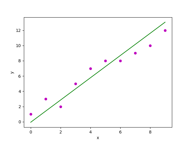
Output of above piece of code is:

Estimated coefficients:
b_0 = -0.0586206896552
b_1 = 1.45747126437

And graph obtained looks like this: