Neural Networks | A beginners guide

Neural networks are artificial systems that were inspired by biological neural networks. These systems learn to perform tasks by being exposed to various datasets and examples without any task-specific rules. The idea is that the system generates identifying characteristics from the data they have been passed without being programmed with a pre-programmed understanding of these datasets.

Neural networks are based on computational models for threshold logic. Threshold logic is a combination of algorithms and mathematics. Neural networks are based either on the study of the brain or on the application of neural networks to artificial intelligence. The work has led to improvements in finite automata theory.

Components of a typical neural network involve neurons, connections, weights, biases, propagation function, and a learning rule. Neurons will receive an input $p_j(t)$ from predecessor neurons that have an activation $a_j(t)$ , threshold $$\theta$_j$ , an activation function f, and an output function $f_{out}$ . Connections consist of connections, weights and biases which rules how neuron $i$ transfers output to neuron $j$ . Propagation computes the input and outputs the output and sums the predecessor neurons function with the weight. The learning rule modifies the weights and thresholds of the variables in the network.

Supervised vs Unsupervised Learning:
Neural networks learn via supervised learning; Supervised machine learning involves an input variable x and output variable y. The algorithm learns from a training dataset. With each correct answers, algorithms iteratively make predictions on the data. The learning stops when the algorithm reaches an acceptable level of performance.
Unsupervised machine learning has input data X and no corresponding output variables. The goal is to model the underlying structure of the data for understanding more about the data. The keywords for supervised machine learning are classification and regression. For unsupervised machine learning, the keywords are clustering and association.

Evolution of Neural Networks:
Hebbian learning deals with neural plasticity. Hebbian learning is unsupervised and deals with long term potentiation. Hebbian learning deals with pattern recognition and exclusive-or circuits; deals with if-then rules.

Back propagation solved the exclusive-or issue that Hebbian learning could not handle. This also allowed for multi-layer networks to be feasible and efficient. If an error was found, the error was solved at each layer by modifying the weights at each node. This led to the development of support vector machines, linear classifiers, and max-pooling. The vanishing gradient problem affects feedforward networks that use back propagation and recurrent neural network. This is known as deep-learning.

Hardware-based designs are used for biophysical simulation and neurotrophic computing. They have large scale component analysis and convolution creates new class of neural computing with analog. This also solved back-propagation for many-layered feedforward neural networks.

Convolutional networks are used for alternating between convolutional layers and max-pooling layers with connected layers (fully or sparsely connected) with a final classification layer. The learning is done without unsupervised pre-training. Each filter is equivalent to a weights vector that has to be trained. The shift variance has to be guaranteed to dealing with small and large neural networks. This is being resolved in Development Networks.

Types of Neural Networks

There are seven types of neural networks that can be used.

The first is a multilayer perceptron which has three or more layers and uses a nonlinear activation function.
The second is the convolutional neural network that uses a variation of the multilayer perceptrons.
The third is the recursive neural network that uses weights to make structured predictions.
The fourth is a recurrent neural network that makes connections between the neurons in a directed cycle. The long short-term memory neural network uses the recurrent neural network architecture and does not use activation function.
The final two are sequence to sequence modules which uses two recurrent networks and shallow neural networks which produces a vector space from an amount of text. These neural networks are applications of the basic neural network demonstrated below.

For the example, the neural network will work with three vectors: a vector of attributes X, a vector of classes Y, and a vector of weights W. The code will use 100 iterations to fit the attributes to the classes. The predictions are generated, weighed, and then outputted after iterating through the vector of weights W. The neural network handles back propagation.

Examples:

Input :
X { 2.6, 3.1, 3.0,
    3.4, 2.1, 2.5,
    2.6, 1.3, 4.9, 
    0.1, 0.3, 2.3,};
y {1, 1, 1};
W {0.3, 0.4, 0.6}; 

Output :
0.990628 
0.984596 
0.994117

Below is the implementations:

import numpy as np 
 
# array of any amount of numbers. n = m 
X = np.array([[1, 2, 3], 
              [3, 4, 1], 
              [2, 5, 3]]) 
               
# multiplication 
y = np.array([[.5, .3, .2]]) 
 
# transpose of y 
y = y.T 
 
# sigma value 
sigm = 2
 
# find the delta 
delt = np.random.random((3, 3)) - 1
 
for j in range(100): 
    # find matrix 1. 100 layers.  
    m1 = (y - (1/(1 + np.exp(-(np.dot((1/(1 + np.exp( 
                   -(np.dot(X, sigm))))), delt))))))*((1/( 
                       1 + np.exp(-(np.dot((1/(1 + np.exp( 
                   -(np.dot(X, sigm))))), delt)))))*(1-(1/( 
                       1 + np.exp(-(np.dot((1/(1 + np.exp( 
                   -(np.dot(X, sigm))))), delt))))))) 
                    
    # find matrix 2 
    m2 = m1.dot(delt.T) * ((1/(1 + np.exp(-(np.dot(X, sigm))))) 
                    * (1-(1/(1 + np.exp(-(np.dot(X, sigm))))))) 
    # find delta 
    delt = delt + (1/(1 + np.exp(-(np.dot(X, sigm))))).T.dot(m1) 
     
    # find sigma 
    sigm = sigm + (X.T.dot(m2)) 
     
# print output from the matrix 
print(1/(1 + np.exp(-(np.dot(X, sigm))))) 

Output:

[[ 0.99999294  0.99999379  0.99999353]
 [ 0.99999987  0.99999989  0.99999988]
 [ 1.          1.          1.        ]]

Limitations:
The neural network is for a supervised model. It does not handle unsupervised machine learning and does not cluster and associate data. It also lacks a level of accuracy that will be found in more computationally expensive neural network. Based on Andrew Trask’s neural network. Also, the neural network does not work with any matrices where X’s number of rows and columns do not match Y and W’s number of rows.

The next steps would be to create an unsupervised neural network and to increase computational power for the supervised model with more iterations and threading.

Resources:

http://neuralnetworksanddeeplearning.com
https://skymind.ai/wiki/neural-network
http://pages.cs.wisc.edu/~bolo/shipyard/neural/local.html
https://iamtrask.github.io/2015/07/12/basic-python-network/

A single neuron neural network in Python

Neural networks are the core of deep learning, a field which has practical applications in many different areas. Today neural networks are used for image classification, speech recognition, object detection etc. Now, Let’s try to understand the basic unit behind all this state of art technique.

A single neuron transforms given input into some output. Depending on the given input and weights assigned to each input, decide whether the neuron fired or not. Let’s assume the neuron has 3 input connections and one output.

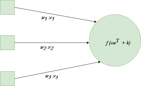
We will be using tanh activation function in given example.

The end goal is to find the optimal set of weights for this neuron which produces correct results. Do this by training the neuron with several different training examples. At each step calculate the error in the output of neuron, and back propagate the gradients. The step of calculating the output of neuron is called forward propagation while calculation of gradients is called back propagation.

Below is the implementation :

# Python program to implement a  
# single neuron neural network 
# import all necessery libraries 
from numpy import exp, array, random, dot, tanh 
# Class to create a neural  
# network with single neuron 
class NeuralNetwork(): 
def __init__(self): 
# Using seed to make sure it'll   
# generate same weights in every run 
random.seed(1) 
# 3x1 Weight matrix 
self.weight_matrix = 2 * random.random((3, 1)) - 1
# tanh as activation fucntion 
def tanh(self, x): 
return tanh(x) 
# derivative of tanh function. 
# Needed to calculate the gradients. 
def tanh_derivative(self, x): 
return 1.0 - tanh(x) ** 2
# forward propagation 
def forward_propagation(self, inputs): 
return self.tanh(dot(inputs, self.weight_matrix)) 
# training the neural network. 
def train(self, train_inputs, train_outputs, 
num_train_iterations): 
# Number of iterations we want to 
# perform for this set of input. 
for iteration in range(num_train_iterations): 
output = self.forward_propagation(train_inputs) 
# Calculate the error in the output. 
error = train_outputs - output 
# multiply the error by input and then  
# by gradient of tanh funtion to calculate 
# the adjustment needs to be made in weights 
adjustment = dot(train_inputs.T, error *
self.tanh_derivative(output)) 
# Adjust the weight matrix 
self.weight_matrix += adjustment 
# Driver Code 
if __name__ == "__main__": 
neural_network = NeuralNetwork() 
print ('Random weights at the start of training') 
print (neural_network.weight_matrix) 
train_inputs = array([[0, 0, 1], [1, 1, 1], [1, 0, 1], [0, 1, 1]]) 
train_outputs = array([[0, 1, 1, 0]]).T 
neural_network.train(train_inputs, train_outputs, 10000) 
print ('New weights after training') 
print (neural_network.weight_matrix) 
# Test the neural network with a new situation. 
print ("Testing network on new examples ->") 
print (neural_network.forward_propagation(array([1, 0, 0]))) 

Output :

Random weights at the start of training
[[-0.16595599]
 [ 0.44064899]
 [-0.99977125]]

New weights after training
[[5.39428067]
 [0.19482422]
 [0.34317086]]

Testing network on new examples ->
[0.99995873]

Activation functions in Neural Networks

It is recommended to understand what is a neural network before reading this article. In The process of building a neural network, one of the choices you get to make is what activation function to use in the hidden layer as well as at the output layer of the network. This article discusses some of the choices.

Elements of a Neural Network :-
Input Layer :- This layer accepts input features. It provides information from the outside world to the network, no computation is performed at this layer, nodes here just pass on the information(features) to the hidden layer.
Hidden Layer :- Nodes of this layer are not exposed to the outer world, they are the part of the abstraction provided by any neural network. Hidden layer performs all sort of computation on the features entered through the input layer and transfer the result to the output layer.
Output Layer :- This layer bring up the information learned by the network to the outer world.

What is an activation function and why to use them?

Definition of activation function:- Activation function decides, whether a neuron should be activated or not by calculating weighted sum and further adding bias with it. The purpose of the activation function is to introduce non-linearity into the output of a neuron.

Explanation :-
We know, neural network has neurons that work in correspondence of weight, bias and their respective activation function. In a neural network, we would update the weights and biases of the neurons on the basis of the error at the output. This process is known as back-propagation. Activation functions make the back-propagation possible since the gradients are supplied along with the error to update the weights and biases.

Why do we need Non-linear activation functions :-
A neural network without an activation function is essentially just a linear regression model. The activation function does the non-linear transformation to the input making it capable to learn and perform more complex tasks.

Mathematical proof :-

Suppose we have a Neural net like this :-

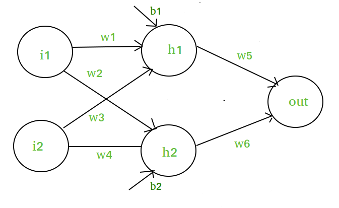
Elements of the diagram :-
Hidden layer i.e. layer 1 :-

z(1) = W(1)X + b(1)
a(1) = z(1)
Here,

z(1) is the vectorized output of layer 1

W(1) be the vectorized weights assigned to neurons
of hidden layer i.e. w1, w2, w3 and w4

X be the vectorized input features i.e. i1 and i2

b is the vectorized bias assigned to neurons in hidden
layer i.e. b1 and b2

a(1) is the vectorized form of any linear function.

(Note: We are not considering activation function here)

Layer 2 i.e. output layer :-

//  Note : Input for layer 
//   2 is output from layer 1
z(2) = W(2)a(1) + b(2)  
a(2) = z(2)

Calculation at Output layer:

// Putting value of z(1) here

z(2) = (W(2) * [W(1)X + b(1)]) + b(2) 

z(2) = [W(2) * W(1)] * X + [W(2)*b(1) + b(2)]

Let, 
    [W(2) * W(1)] = W
    [W(2)*b(1) + b(2)] = b

Final output : z(2) = W*X + b
Which is again a linear function

This observation results again in a linear function even after applying a hidden layer, hence we can conclude that, doesn’t matter how many hidden layer we attach in neural net, all layers will behave same way because the composition of two linear function is a linear function itself. Neuron can not learn with just a linear function attached to it. A non-linear activation function will let it learn as per the difference w.r.t error.
Hence we need activation function.

VARIANTS OF ACTIVATION FUNCTION :-

1). Linear Function :-

Equation : Linear function has the equation similar to as of a straight line i.e. y = ax
No matter how many layers we have, if all are linear in nature, the final activation function of last layer is nothing but just a linear function of the input of first layer.
Range : -inf to +inf
Uses : Linear activation function is used at just one place i.e. output layer.
Issues : If we will differentiate linear function to bring non-linearity, result will no more depend on input “x” and function will become constant, it won’t introduce any ground-breaking behavior to our algorithm.

For example : Calculation of price of a house is a regression problem. House price may have any big/small value, so we can apply linear activation at output layer. Even in this case neural net must have any non-linear function at hidden layers.

2). Sigmoid Function :-

It is a function which is plotted as ‘S’ shaped graph.
Equation :
A = 1/(1 + e^-x)
Nature : Non-linear. Notice that X values lies between -2 to 2, Y values are very steep. This means, small changes in x would also bring about large changes in the value of Y.
Value Range : 0 to 1
Uses : Usually used in output layer of a binary classification, where result is either 0 or 1, as value for sigmoid function lies between 0 and 1 only so, result can be predicted easily to be 1 if value is greater than 0.5 and 0 otherwise.

3). Tanh Function :- The activation that works almost always better than sigmoid function is Tanh function also knows as Tangent Hyperbolic function. It’s actually mathematically shifted version of the sigmoid function. Both are similar and can be derived from each other.

Equation :-

f(x) = tanh(x) = 2/(1 + e^-2x) - 1
OR
tanh(x) = 2 * sigmoid(2x) - 1

- Value Range :- -1 to +1
- Nature :- non-linear
- Uses :- Usually used in hidden layers of a neural network as it’s values lies between -1 to 1 hence the mean for the hidden layer comes out be 0 or very close to it, hence helps in centering the data by bringing mean close to 0. This makes learning for the next layer much easier.

4). RELU :- Stands for Rectified linear unit. It is the most widely used activation function. Chiefly implemented in hidden layers of Neural network.

Equation :- A(x) = max(0,x). It gives an output x if x is positive and 0 otherwise.
Value Range :- [0, inf)
Nature :- non-linear, which means we can easily backpropagate the errors and have multiple layers of neurons being activated by the ReLU function.
Uses :- ReLu is less computationally expensive than tanh and sigmoid because it involves simpler mathematical operations. At a time only a few neurons are activated making the network sparse making it efficient and easy for computation.

In simple words, RELU learns much faster than sigmoid and Tanh function.

5). Softmax Function :- The softmax function is also a type of sigmoid function but is handy when we are trying to handle classification problems.

- Nature :- non-linear
- Uses :- Usually used when trying to handle multiple classes. The softmax function would squeeze the outputs for each class between 0 and 1 and would also divide by the sum of the outputs.
- Ouput:- The softmax function is ideally used in the output layer of the classifier where we are actually trying to attain the probabilities to define the class of each input.

CHOOSING THE RIGHT ACTIVATION FUNCTION

The basic rule of thumb is if you really don’t know what activation function to use, then simply use RELU as it is a general activation function and is used in most cases these days.
If your output is for binary classification then, sigmoid function is very natural choice for output layer.

Foot Note :-
The activation function does the non-linear transformation to the input making it capable to learn and perform more complex tasks.

Reference :
Understanding Activation Functions in Neural Networks

##########################################

# Python program to implement a
# single neuron neural network

# import all necessery libraries
from numpy import exp, array, random, dot, tanh

# Class to create a neural
# network with single neuron
class NeuralNetwork():

def __init__(self):

# Using seed to make sure it'll
# generate same weights in every run
random.seed(1)

# 3x1 Weight matrix
self.weight_matrix = 2 * random.random((3, 1)) - 1

# tanh as activation fucntion
def tanh(self, x):
return tanh(x)

# derivative of tanh function.
# Needed to calculate the gradients.
def tanh_derivative(self, x):
return 1.0 - tanh(x) ** 2

# forward propagation
def forward_propagation(self, inputs):
return self.tanh(dot(inputs, self.weight_matrix))

# training the neural network.
def train(self, train_inputs, train_outputs,
num_train_iterations):

# Number of iterations we want to
# perform for this set of input.
for iteration in range(num_train_iterations):
output = self.forward_propagation(train_inputs)

# Calculate the error in the output.
error = train_outputs - output

# multiply the error by input and then
# by gradient of tanh funtion to calculate
# the adjustment needs to be made in weights
adjustment = dot(train_inputs.T, error *
self.tanh_derivative(output))

# Adjust the weight matrix
self.weight_matrix += adjustment

# Driver Code
if __name__ == "__main__":

neural_network = NeuralNetwork()

print ('Random weights at the start of training')
print (neural_network.weight_matrix)

train_inputs = array([[0, 0, 1], [1, 1, 1], [1, 0, 1], [0, 1, 1]])
train_outputs = array([[0, 1, 1, 0]]).T

neural_network.train(train_inputs, train_outputs, 10000)

print ('New weights after training')
print (neural_network.weight_matrix)

# Test the neural network with a new situation.
print ("Testing network on new examples ->")
print (neural_network.forward_propagation(array([1, 0, 0])))