
Introduction to TensorFlow
This article is a brief introduction to TensorFlow library using Python programming language.
Introduction
TensorFlow is an open-source software library. TensorFlow was originally developed by researchers and engineers working on the Google Brain Team within Google’s Machine Intelligence research organization for the purposes of conducting machine learning and deep neural networks research, but the system is general enough to be applicable in a wide variety of other domains as well!
Let us first try to understand what the word TensorFlow actually mean!
TensorFlow is basically a software library for numerical computation using data flow graphs where:
- nodes in the graph represent mathematical operations.
- edges in the graph represent the multidimensional data arrays (called tensors) communicated between them. (Please note that tensor is the central unit of data in TensorFlow).
Consider the diagram given below:
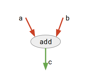
Here, add is a node which represents addition operation. a and b are input tensors and c is the resultant tensor.
This flexible architecture allows you to deploy computation to one or more CPUs or GPUs in a desktop, server, or mobile device with a single API!
TensorFlow APIs
TensorFlow provides multiple APIs (Application Programming Interfaces). These can be classified into 2 major categories:
- Low level API:
- complete programming control
- recommended for machine learning researchers
- provides fine levels of control over the models
- TensorFlow Core is the low level API of TensorFlow.
- High level API:
- built on top of TensorFlow Core
- easier to learn and use than TensorFlow Core
- make repetitive tasks easier and more consistent between different users
- tf.contrib.learn is an example of a high level API.
In this article, we first discuss the basics of TensorFlow Core and then explore the higher level API, tf.contrib.learn.
TensorFlow Core
1. Installing TensorFlow
An easy to follow guide for TensorFlow installation is available here:
Installing TensorFlow.
Once installed, you can ensure a successful installation by running this command in python interpreter:
import tensorflow as tf
2. The Computational Graph
Any TensorFlow Core program can be divided into two discrete sections:
- Building the computational graph.A computational graph is nothing but a series of TensorFlow operations arranged into a graph of nodes.
- Running the computational graph.To actually evaluate the nodes, we must run the computational graph within a session. A session encapsulates the control and state of the TensorFlow runtime.
Now, let us write our very first TensorFlow program to understand above concept:
# importing tensorflow import tensorflow as tf # creating nodes in computation graph node1 = tf.constant(3, dtype=tf.int32) node2 = tf.constant(5, dtype=tf.int32) node3 = tf.add(node1, node2) # create tensorflow session object sess = tf.Session() # evaluating node3 and printing the result print("Sum of node1 and node2 is:",sess.run(node3)) # closing the session sess.close() |
Output:
Sum of node1 and node2 is: 8
Let us try to understand above code:
- Step 1 : Create a computational graph
By creating computational graph, we mean defining the nodes. Tensorflow provides different types of nodes for a variety of tasks. Each node takes zero or more tensors as inputs and produces a tensor as an output.- In above program, the nodes node1 and node2 are of tf.constant type. A constant node takes no inputs, and it outputs a value it stores internally. Note that we can also specify the data type of output tensor using dtype argument.
node1 = tf.constant(3, dtype=tf.int32)
node2 = tf.constant(5, dtype=tf.int32)
- node3 is of tf.add type. It takes two tensors as input and returns their sum as output tensor.
node3 = tf.add(node1, node2)
- In above program, the nodes node1 and node2 are of tf.constant type. A constant node takes no inputs, and it outputs a value it stores internally. Note that we can also specify the data type of output tensor using dtype argument.
- Step 2 : Run the computational graph
In order to run the computational graph, we need to create a session. To create a session, we simply do:sess = tf.Session()
Now, we can invoke the run method of session object to perform computations on any node:
print("Sum of node1 and node2 is:",sess.run(node3))Here, node3 gets evaluated which further invokes node1 and node2. Finally, we close the session using:
sess.close()
Note: Another(and better) method of working with sessions is to use with block like this:
with tf.Session() as sess:
    print("Sum of node1 and node2 is:",sess.run(node3))
The benefit of this approach is that you do not need to close the session explicitly as it gets automatically closed once control goes out of the scope of with block.
3. Variables
TensorFlow has Variable nodes too which can hold variable data. They are mainly used to hold and update parameters of a training model.
Variables are in-memory buffers containing tensors. They must be explicitly initialized and can be saved to disk during and after training. You can later restore saved values to exercise or analyze the model.
An important difference to note between a constant and Variable is:
A constant’s value is stored in the graph and its value is replicated wherever the graph is loaded. A variable is stored separately, and may live on a parameter server.
Given below is an example using Variable:
# importing tensorflow import tensorflow as tf # creating nodes in computation graph node = tf.Variable(tf.zeros([2,2])) # running computation graph with tf.Session() as sess: # initialize all global variables sess.run(tf.global_variables_initializer()) # evaluating node print("Tensor value before addition:\n",sess.run(node)) # elementwise addition to tensor node = node.assign(node + tf.ones([2,2])) # evaluate node again print("Tensor value after addition:\n", sess.run(node)) |
Output:
Tensor value before addition:
 [[ 0.  0.]
 [ 0.  0.]]
Tensor value after addition:
 [[ 1.  1.]
 [ 1.  1.]]
In above program:
- We define a node of type Variable and assign it some initial value.
node = tf.Variable(tf.zeros([2,2]))
- To initialize the variable node in current session’s scope, we do:
sess.run(tf.global_variables_initializer())
- To assign a new value to a variable node, we can use assign method like this:
node = node.assign(node + tf.ones([2,2]))
4. Placeholders
A graph can be parameterized to accept external inputs, known as placeholders. A placeholder is a promise to provide a value later.
While evaluating the graph involving placeholder nodes, a feed_dict parameter is passed to the session’s run method to specify Tensors that provide concrete values to these placeholders.
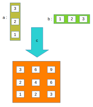
Consider the example given below:
# importing tensorflow import tensorflow as tf # creating nodes in computation graph a = tf.placeholder(tf.int32, shape=(3,1)) b = tf.placeholder(tf.int32, shape=(1,3)) c = tf.matmul(a,b) # running computation graph with tf.Session() as sess: print(sess.run(c, feed_dict={a:[[3],[2],[1]], b:[[1,2,3]]})) |
Output:
[[3 6 9]
 [2 4 6]
 [1 2 3]]
Let us try to understand above program:
- We define placeholder nodes a and b like this:
a = tf.placeholder(tf.int32, shape=(3,1))
b = tf.placeholder(tf.int32, shape=(1,3))
The first argument is the data type of the tensor and one of the optional argument is shape of the tensor.
- We define another node c which does the operation of matrix multiplication (matmul). We pass the two placeholder nodes as argument.
c = tf.matmul(a,b)
- Finally, when we run the session, we pass the value of placeholder nodes in feed_dict argument of sess.run:
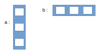
print(sess.run(c, feed_dict={a:[[3],[2],[1]], b:[[1,2,3]]}))Consider the diagrams shown below to clear the concept:
- Initially:
- After sess.run:
5. An example : Linear Regression model
Given below is an implementation of a Linear Regression model using TensorFlow Core API.
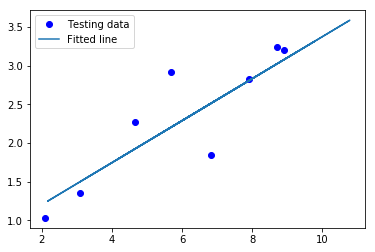
# importing the dependencies import tensorflow as tf import numpy as np import matplotlib.pyplot as plt # Model Parameters learning_rate = 0.01training_epochs = 2000display_step = 200 # Training Data train_X = np.asarray([3.3,4.4,5.5,6.71,6.93,4.168,9.779,6.182,7.59,2.167, 7.042,10.791,5.313,7.997,5.654,9.27,3.1]) train_y = np.asarray([1.7,2.76,2.09,3.19,1.694,1.573,3.366,2.596,2.53,1.221, 2.827,3.465,1.65,2.904,2.42,2.94,1.3]) n_samples = train_X.shape[0] # Test Data test_X = np.asarray([6.83, 4.668, 8.9, 7.91, 5.7, 8.7, 3.1, 2.1]) test_y = np.asarray([1.84, 2.273, 3.2, 2.831, 2.92, 3.24, 1.35, 1.03]) # Set placeholders for feature and target vectors X = tf.placeholder(tf.float32) y = tf.placeholder(tf.float32) # Set model weights and bias W = tf.Variable(np.random.randn(), name="weight") b = tf.Variable(np.random.randn(), name="bias") # Construct a linear model linear_model = W*X + b # Mean squared error cost = tf.reduce_sum(tf.square(linear_model - y)) / (2*n_samples) # Gradient descent optimizer = tf.train.GradientDescentOptimizer(learning_rate).minimize(cost) # Initializing the variables init = tf.global_variables_initializer() # Launch the graph with tf.Session() as sess: # Load initialized variables in current session sess.run(init) # Fit all training data for epoch in range(training_epochs): # perform gradient descent step sess.run(optimizer, feed_dict={X: train_X, y: train_y}) # Display logs per epoch step if (epoch+1) % display_step == 0: c = sess.run(cost, feed_dict={X: train_X, y: train_y}) print("Epoch:{0:6} \t Cost:{1:10.4} \t W:{2:6.4} \t b:{3:6.4}". format(epoch+1, c, sess.run(W), sess.run(b))) # Print final parameter values print("Optimization Finished!") training_cost = sess.run(cost, feed_dict={X: train_X, y: train_y}) print("Final training cost:", training_cost, "W:", sess.run(W), "b:", sess.run(b), '\n') # Graphic display plt.plot(train_X, train_y, 'ro', label='Original data') plt.plot(train_X, sess.run(W) * train_X + sess.run(b), label='Fitted line') plt.legend() plt.show() # Testing the model testing_cost = sess.run(tf.reduce_sum(tf.square(linear_model - y)) / (2 * test_X.shape[0]), feed_dict={X: test_X, y: test_y}) print("Final testing cost:", testing_cost) print("Absolute mean square loss difference:", abs(training_cost - testing_cost)) # Display fitted line on test data plt.plot(test_X, test_y, 'bo', label='Testing data') plt.plot(train_X, sess.run(W) * train_X + sess.run(b), label='Fitted line') plt.legend() plt.show() |
Epoch: 200 Cost: 0.1715 W: 0.426 b:-0.4371 Epoch: 400 Cost: 0.1351 W:0.3884 b:-0.1706 Epoch: 600 Cost: 0.1127 W:0.3589 b:0.03849 Epoch: 800 Cost: 0.09894 W:0.3358 b:0.2025 Epoch: 1000 Cost: 0.09047 W:0.3176 b:0.3311 Epoch: 1200 Cost: 0.08526 W:0.3034 b:0.4319 Epoch: 1400 Cost: 0.08205 W:0.2922 b:0.5111 Epoch: 1600 Cost: 0.08008 W:0.2835 b:0.5731 Epoch: 1800 Cost: 0.07887 W:0.2766 b:0.6218 Epoch: 2000 Cost: 0.07812 W:0.2712 b: 0.66 Optimization Finished! Final training cost: 0.0781221 W: 0.271219 b: 0.65996Final testing cost: 0.0756337 Absolute mean square loss difference: 0.00248838
Let us try to understand the above code.
- First of all, we define some parameters for training our model, like:
learning_rate = 0.01
training_epochs = 2000
display_step = 200
- Then we define placeholder nodes for feature and target vector.
X = tf.placeholder(tf.float32)
y = tf.placeholder(tf.float32)
- Then, we define variable nodes for weight and bias.
W = tf.Variable(np.random.randn(), name="weight")
b = tf.Variable(np.random.randn(), name="bias")
- linear_model is an operational node which calculates the hypothesis for the linear regression model.
linear_model = W*X + b
- Loss (or cost) per gradient descent is calculated as the mean squared error and its node is defined as:
cost = tf.reduce_sum(tf.square(linear_model - y)) / (2*n_samples)
- Finally, we have the optimizer node which implements the Gradient Descent Algorithm.
optimizer = tf.train.GradientDescentOptimizer(learning_rate).minimize(cost)
- Now, the training data is fit into the linear model by applying the Gradient Descent Algorithm. The task is repeated training_epochs number of times. In each epoch, we perform the gradient descent step like this:
sess.run(optimizer, feed_dict={X: train_X, y: train_y}) - After every display_step number of epochs, we print the value of current loss which is found using:
c = sess.run(cost, feed_dict={X: train_X, y: train_y}) - The model is evaluated on test data and testing_cost is calculated using:
testing_cost = sess.run(tf.reduce_sum(tf.square(linear_model - y)) / (2 * test_X.shape[0]),
                          feed_dict={X: test_X, y: test_y})
tf.contrib.learn
tf.contrib.learn is a high-level TensorFlow library that simplifies the mechanics of machine learning, including the following:
- running training loops
- running evaluation loops
- managing data sets
- managing feeding
Let us try to see the implementation of Linear regression on same data we used above using tf.contrib.learn.
# importing the dependencies import tensorflow as tf import numpy as np # declaring list of features features = [tf.contrib.layers.real_valued_column("X")] # creating a linear regression estimator estimator = tf.contrib.learn.LinearRegressor(feature_columns=features) # training and test data train_X = np.asarray([3.3,4.4,5.5,6.71,6.93,4.168,9.779,6.182,7.59,2.167, 7.042,10.791,5.313,7.997,5.654,9.27,3.1]) train_y = np.asarray([1.7,2.76,2.09,3.19,1.694,1.573,3.366,2.596,2.53,1.221, 2.827,3.465,1.65,2.904,2.42,2.94,1.3]) test_X = np.asarray([6.83, 4.668, 8.9, 7.91, 5.7, 8.7, 3.1, 2.1]) test_y = np.asarray([1.84, 2.273, 3.2, 2.831, 2.92, 3.24, 1.35, 1.03]) # function to feed dict of numpy arrays into the model for training input_fn = tf.contrib.learn.io.numpy_input_fn({"X":train_X}, train_y, batch_size=4, num_epochs=2000) # function to feed dict of numpy arrays into the model for testing test_input_fn = tf.contrib.learn.io.numpy_input_fn({"X":test_X}, test_y) # fit training data into estimator estimator.fit(input_fn=input_fn) # print value of weight and bias W = estimator.get_variable_value('linear/X/weight')[0][0] b = estimator.get_variable_value('linear/bias_weight')[0] print("W:", W, "\tb:", b) # evaluating the final loss train_loss = estimator.evaluate(input_fn=input_fn)['loss'] test_loss = estimator.evaluate(input_fn=test_input_fn)['loss'] print("Final training loss:", train_loss) print("Final testing loss:", test_loss) |
W: 0.252928     b: 0.802972
Final training loss: 0.153998
Final testing loss: 0.0777036
Let us try to understand the above code.
- The shape and type of feature matrix is declared using a list. Each element of the list defines the structure of a column. In above example, we have only 1 feature which stores real values and has been given a name X.
features = [tf.contrib.layers.real_valued_column("X")] - Then, we need an estimator. An estimator is nothing but a pre-defined model with many useful methods and parameters. In above example, we use a Linear Regression model estimator.
estimator = tf.contrib.learn.LinearRegressor(feature_columns=features)
- For training purpose, we need to use an input function which is responsible for feeding data to estimator while training. It takes the feature column values as dictionary. Many other parameters like batch size, number of epochs, etc can be specified.
input_fn = tf.contrib.learn.io.numpy_input_fn({"X":train_X}, train_y, batch_size=4, num_epochs=2000) - To fit training data to estimator, we simply use fit method of estimator in which input function is passed as an argument.
estimator.fit(input_fn=input_fn)
- Once training is complete, we can get the value of different variables using get_variable_value method of estimator. You can get a list of all variables using get_variable_names method.
W = estimator.get_variable_value('linear/X/weight')[0][0] b = estimator.get_variable_value('linear/bias_weight')[0] - The mean squared error/loss can be computed as:
train_loss = estimator.evaluate(input_fn=input_fn)['loss']
test_loss = estimator.evaluate(input_fn=test_input_fn)['loss']
This brings us to the end of this Introduction to TensorFlow article!
From here, you can try to explore this tutorial: MNIST For ML Beginners.